Lecture 10

Cluster Analysis

Nick Knowlton

Cluster Analysis

What changes in an unsupervised problem?

  • So far, regression and classification have started with a known response or known class labels.
  • In supervised learning, we use those known outcomes to fit a prediction rule.
  • In clustering, the groups are unknown, so the first question is whether meaningful structure exists at all.
  • That is why similarity or dissimilarity becomes the modelling choice.
  • Different clustering algorithms make different assumptions about the data structure.
    • Hierarchical clustering gives a nested tree.
    • K-means gives compact partitions.
    • K-medoids swaps means for representative observations.
    • DBSCAN keeps dense shapes and leaves sparse points as noise.

Lecture roadmap

  1. Review distance ideas for multivariate data.
  2. Use PCA and UMAP as display maps for data.
  3. Build and interpret a hierarchical clustering tree.
  4. Compare centroid, medoid, and density-based clustering.
  5. Finish by comparing today’s methods on a shared 2D data display.

Synthetic dataset

  • synthetic_points: 118 lecture-generated two-dimensional observations with blobs, an ellipse, a crescent, a ring, and noise.

The ring, crescent, blobs, ellipse, and noise are chosen on purpose: they let us see that no single clustering method handles every geometry equally well. The widgets use the same broad shapes, but they subsample points so each step remains legible on a slide.

Dissimilarity matrices

Minkowski distance: \[ d_{st}^{(q)} = \left(\sum_{j=1}^{p} |x_{sj} - x_{tj}|^q\right)^{1/q}, \qquad q \ge 1. \]

\(q\) value Interpretation
1 Manhattan distance
2 Euclidean distance
Larger \(q\) Larger coordinate differences receive more weight

Example distance matrix

D&D Monsters dataset

monsters: the TidyTuesday D&D Monsters data from 2025-05-27.

  • Each row is a monster, with a type label plus combat features like Strength, Dexterity, HP, challenge rating, and speed.
  • We will cluster on the numeric features, then use type afterward to help interpret the fitted groups.
  • The dataset has 1,000 monsters and 16 numeric features, so we will use dimension reduction to visualize the clusters in two dimensions.

To Scale or not to Scale?

Show code
monster_scale_compare |>
  ggplot(aes(x = value, y = feature, fill = scale_state)) +
  geom_vline(
    data = tibble(scale_state = "Z-score scaled", xint = 0),
    aes(xintercept = xint),
    inherit.aes = FALSE,
    linewidth = 0.7,
    linetype = "dashed",
    colour = "#8a3324"
  ) +
  geom_boxplot(outlier.alpha = 0.2, width = 0.7, orientation = "y") +
  facet_wrap(~ scale_state, ncol = 1, scales = "free_x") +
  guides(fill = "none") +
  labs(x = "Raw units / z-score", y = NULL)

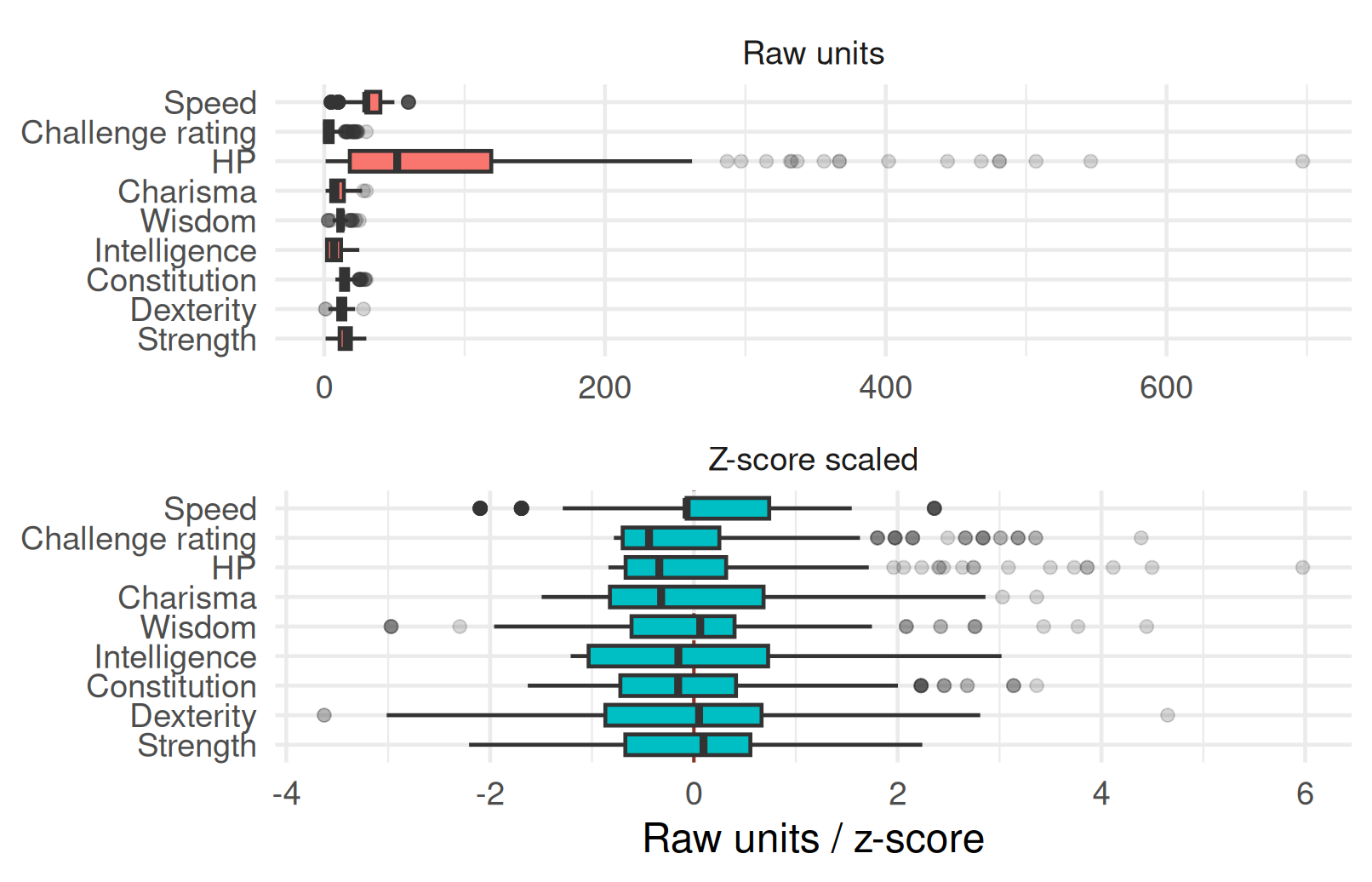
  • The D&D ability scores live on a small scale, while hp_number, cr, and speed_base_number are much larger in raw units.
  • If we cluster on raw Euclidean distance, the large-scale variables dominate the smaller ones.
  • So the clustering examples below use z-score standardization before computing Euclidean distances.
  • Here scale() means subtract the column mean and divide by the column standard deviation, not min-max scaling.

Dimension reduction for visualization

PCA

  • PCA is a linear way to visualize high-dimensional numeric data in just a few coordinates.
  • It chooses orthogonal directions that capture as much variance as possible, so PC1 explains the biggest spread and PC2 explains the next biggest spread.
  • PCA is a projection method, so it can be used as a display map for any clustering method that uses Euclidean distance.

UMAP

  • UMAP is nonlinear and aims to keep nearby points nearby in the 2D map.
  • It is often useful when local neighborhood structure matters more than a single global linear projection.

Monster projections: PCA and UMAP

Hover a monster type or a point to highlight that type in both panels at once. If uwot is unavailable during rendering, the PCA panel still appears and the UMAP panel explains that the embedding is missing.

Hierarchical Clustering

Agglomerative hierarchical clustering

  1. Start with each observation in its own cluster.
  2. Find the closest pair of clusters.
  3. Merge them.
  4. Repeat until only one cluster remains.

There are several ways to define closest when we are comparing clusters rather than individual observations.

  • This is separate from the original point-to-point distance metric.
  • It controls how the clusters are merged.
  • Single linkage uses the closest pair of observations across two clusters.
  • Complete linkage uses the furthest pair of observations across two clusters.
  • Average linkage uses the mean pairwise distance across the two clusters.

Hierarchical clustering on monsters

  • The result is a nested tree of clusters, called a dendrogram.
  • The tree can be cut at different heights to give different clusterings.
Show code
plot(
  monster_hc,
  labels = FALSE,
  hang = -1,
  main = "D&D Monsters dendrogram",
  xlab = "Monsters in leaf order",
  ylab = "Merge dissimilarity",
  sub = ""
)
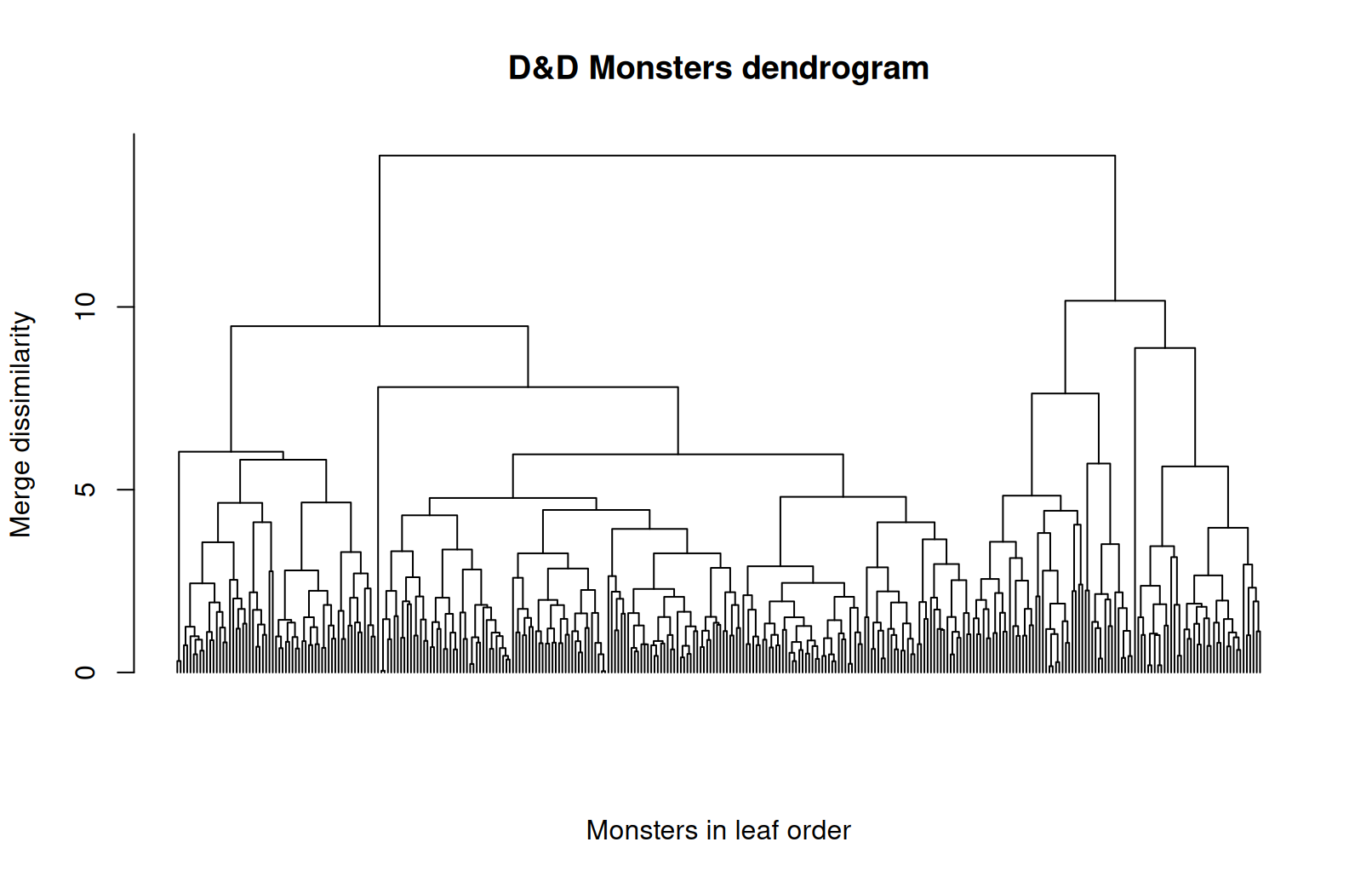
  • The leaves on the x-axis are the individual monsters in the tree order.
  • The height on the y-axis is the dissimilarity at which two clusters merge.

Interactivly building a hierarchical cluster

  • Keep the points fixed and change only the linkage rule.
  • Because “closest clusters” is defined differently, the merge order changes.
  • If you cut the tree at a fixed height later, those different merge histories can lead to different clusterings.

Linkage is not a minor detail

  • Single linkage is sensitive to chains of points.
  • Complete linkage prefers tight, compact groups.
  • Average linkage usually sits between them.

Cutting the tree gives an actual partition

  • cutree(monster_hc, k = 5) turns the hierarchy into five explicit cluster labels.
  • Cutting higher or lower would give a different number of clusters.
  • Move the cut-height slider to see how the partition changes as the horizontal cut moves up or down.
  • The horizontal line shows the active cut height on the dendrogram.
  • Point colours show the resulting subgroup labels at that height on the same projection used elsewhere in the lecture.
  • Lower cuts produce more clusters; higher cuts merge groups into fewer clusters.

Are the clusters stable?

  • After choosing a linkage rule and a tree cut, we can ask whether those same clusters would reappear if the data shifted slightly.
  • Resample observations with replacement to create a new dataset of the same size, then repeat the clustering on that new dataset.
  • Refit the clustering on each resample.
  • Compare the resulting partition with the original.
  • A stable cluster should survive small perturbations to the data.

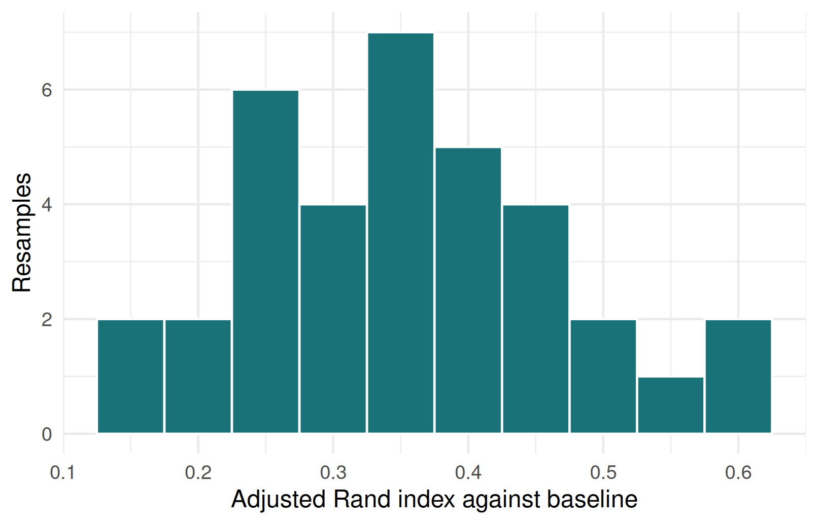
Bootstrap stability on monsters

  • A bootstrap sample is a new dataset made by sampling the monsters with replacement from the original data.
  • The tibble below contains one adjusted Rand index (ARI) value per bootstrap resample; here we used 35 resamples.
  • The adjusted Rand index compares every pair of monsters across two partitions: did that pair stay together, or stay apart, in both clusterings? It then subtracts the agreement expected by chance, \[ \mathrm{ARI} = \frac{\sum_{ij}\binom{n_{ij}}{2} - E}{\frac{1}{2}\left[\sum_i \binom{a_i}{2} + \sum_j \binom{b_j}{2}\right] - E}, \] so 1 means a perfect match to the baseline clustering, 0 means about as much agreement as random assignment, and negative values mean worse than random agreement. Higher values mean more stable cluster structure.

Interactive resampling stability widget

The matrix uses colour for the baseline cluster and transparency for how often a pair of monsters stays together across the summary resamples. The bars on the right summarise average within-cluster stability, so wider bars mean a cluster stays together more consistently.

K-means and K-medoids

K-means minimises within-cluster variation

  • K-means chooses cluster assignments and centroids to minimise the total within-cluster sum of squares.

For Euclidean distance the objective is \[ \sum_{k=1}^K \sum_{C(i)=k} \lVert x_i - \mu_k \rVert^2. \]

Algorithm:

  1. Start by placing the centroids arbitrarily.
  2. Assign each point to the nearest centroid.
  3. Recompute centroids.
  4. Repeat until the centroids reach convergence.

K-means on monsters

K-medoids / PAM

  • PAM stands for Partitioning Around Medoids.
  • Replace the centroid with a real observation, the medoid.
  • This makes the method less sensitive to outliers.
  • It also lets us use any dissimilarity, not just Euclidean distance.

For a dissimilarity matrix, PAM chooses the set of \(K\) medoids that minimizes total assignment dissimilarity: \[ M^* = \arg\min_{M: |M| = K} \sum_{i=1}^n \min_{m \in M} d(i,m). \]

Algorithm:

  1. Start with \(K\) candidate medoids.
  2. Assign each observation to its nearest medoid.
  3. Propose swapping a medoid with a non-medoid.
  4. Accept the swap if the objective decreases; repeat until no improving swap remains.

Interactive K-means versus K-medoids

Switch between methods to compare how centroids and medoids react to bridge points and borderline observations.

Silhouette widths for PAM

A silhouette is a diagnostic for how well an observation fits into its assigned cluster compared to the next best alternative.

  • A silhouette asks whether a point is closer to its own cluster than to a nearby competing cluster.
  • Values near 1 indicate a well-matched point.
  • Values near 0 indicate a boundary point.
  • Negative values suggest the point may fit better in another cluster.
  • Silhouettes are a general clustering diagnostic, not something unique to PAM.
  • Use the K control to compare the PAM silhouettes for 2 through 5 clusters.

PAM diagnostic: choosing K

Use K = 2 through 5 and switch between PCA and UMAP to compare the final PAM clustering with its silhouette diagnostic. Hover a silhouette bar or a plotted monster to link the same observation across both panels.

When K-means and PAM disagree

Agreement Count Percent
Same cluster after relabelling 233 70.6%
Different cluster 97 29.4%

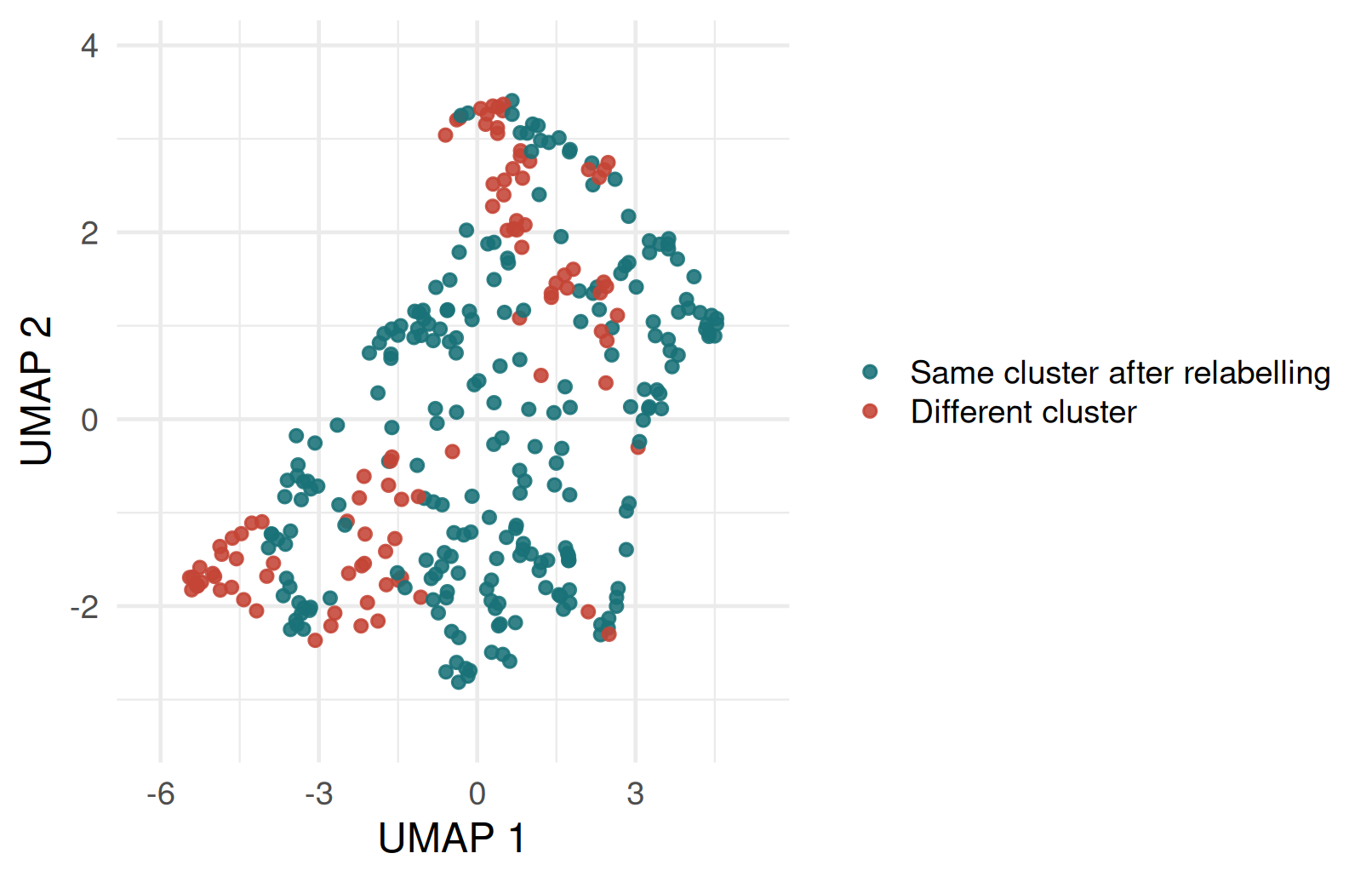
  • Disagreement usually shows up around boundary observations or points affected by outliers.
  • K-means is faster and works well for compact numeric clusters.
  • PAM is more robust when the center should be a real observation or when outliers matter.

Disagreement across K values

Use K = 2 through 5 to see where K-means and PAM disagree after relabelling PAM clusters to the closest K-means labels. Disagreements are highlighted strongly; agreements stay visible as context.

Density Clustering

Clustering by density: DBSCAN

DBSCAN stands for Density-Based Spatial Clustering of Applications with Noise.

  • It groups points that are packed closely together (densely) and labels isolated points as noise.

  • Unlike K-means, DBSCAN does not require us to choose the number of clusters in advance, and it can recover irregular shapes such as rings, crescents, or curved bands.

Advantages:

  • Can find clusters of arbitrary shape.
  • Can identify noise points that do not belong to any cluster.

Disadvantages:

  • Sensitive to the choice of parameters (eps and MinPts).

Terms to know:

  • Core point: at least MinPts observations in its eps-neighborhood.
  • Border point: not core, but within the neighborhood of a core point.
  • Noise point: neither core nor border.
  • eps or epsilon: the neighborhood radius around a point.
  • MinPts: the minimum number of observations in the epsilon-neighborhood needed for a core point. Here that count includes the point itself.

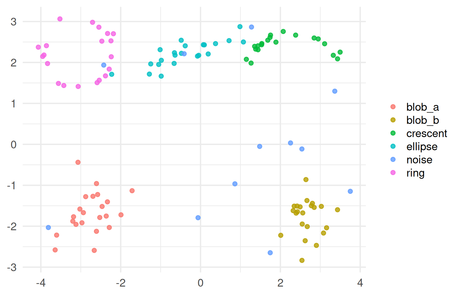
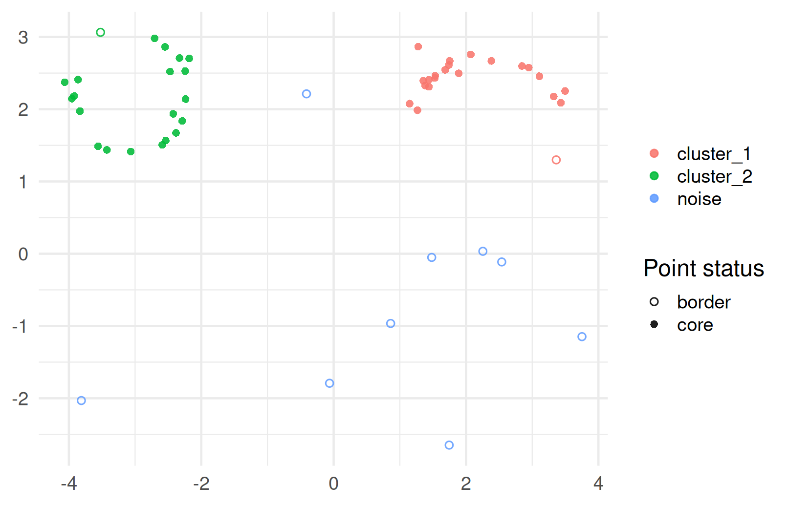
DBSCAN on our ring/crescent data

  • This is exactly the kind of geometry where centroid-based methods tend to struggle.
  • The ring and crescent are useful because they show how density-based clustering can recover non-convex shapes.
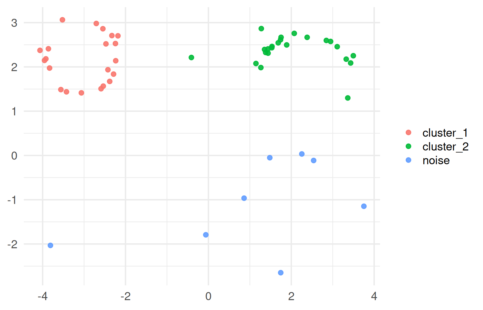
Show code
ggplot(dbscan_plot_data, aes(x = x, y = y, colour = cluster, shape = point_type)) +
  geom_point(size = 2.2, alpha = 0.88) +
  scale_shape_manual(values = c(core = 16, border = 1, noise = 4)) +
  labs(x = NULL, y = NULL, colour = NULL, shape = "Point status")

Interactive DBSCAN widget

DBSCAN repeats: inspect an unvisited point, test whether it is core, expand through its neighbors if it is core, and otherwise leave it as provisional noise until a later core point reaches it.

HDBSCAN

HDBSCAN stands for Hierarchical Density-Based Spatial Clustering of Applications with Noise.

  • The “H” in HDBSCAN stands for “hierarchical,” which means it builds a hierarchy of clusters based on varying density thresholds.
Show code
if (is.null(hdbscan_plot_data)) {
  tibble(status = "Install the dbscan package to render the HDBSCAN example.")
} else {
  ggplot(hdbscan_plot_data, aes(x = x, y = y, colour = cluster)) +
    geom_point(alpha = 0.9, size = 2.2) +
    labs(x = NULL, y = NULL, colour = NULL)
}

Advantages:

  • Can handle clusters of varying densities better than DBSCAN.
  • Provides a more robust clustering solution when the data contains clusters of different densities.

Disadvantages:

  • More complex than DBSCAN and may require more computational resources.
  • Like DBSCAN, it can be sensitive to parameter choices, although it has fewer parameters to tune.

Wrapping up: comparing methods on the same display

Monsters clustered using today’s methods

For hierarchical clustering, K-means, and PAM, the cluster count is chosen by us. For DBSCAN, eps and MinPts are inputs and the number of clusters is an output.

Practical comparison

Method Strength Risk Needs scaling?
Hierarchical Full tree, no need to pre-fix K Linkage choice matters Usually yes
K-means Fast, familiar, easy to explain Splits non-convex shapes Yes
K-medoids Robust, medoids are real points Slower than K-means Usually yes
DBSCAN Handles noise and shape Parameter tuning can be awkward Yes
HDBSCAN Better with varying density Less intuitive Yes

Chapter 7 of the course notes covers Gower dissimilarity, bootstrap stability, HDBSCAN, and UMAP with more mathematical detail.