Lecture 11

Association Rule Mining

What are Association Rules?

Discovering interesting relationships among items in large collections of transactions.

Classic framing: market basket analysis

• Supermarket receipts
• Online shopping carts

But also:

• Recipe ingredients 🍕
• Medical symptoms → diagnoses
• Web page visits → next click
• Survey question response patterns

The question:

“If a recipe uses garlic and olive oil, what other ingredients does it tend to include?”

An association rule has the form:

\[\{garlic, olive\_oil\} \Rightarrow \{parmesan\}\]

• Antecedent (left-hand side): condition
• Consequent (right-hand side): associated item

Transactions as a Binary Matrix

Each transaction is a set of items. We represent the data as a binary matrix:

• Rows = transactions (recipes, shopping trips, patients)
• Columns = items
• Cell = 1 if item present, 0 otherwise

Key insight

Association rules work on presence/absence data — no quantities, no order. Just “was it in the basket or not?”

Let’s build one interactively…

Widget 1: Transaction Builder

Toggle pizza toppings on and off to build a transaction database. Watch the binary matrix and item frequencies update in real time.

import { transactionBuilderWidget } from "./widgets/association-rules/transaction-builder-widget.js"
viewof pizzaToggles = transactionBuilderWidget()

Support, Confidence, and Lift

The three key metrics for evaluating association rules:

Support

How frequently the itemset appears:

\[\text{supp}(A \Rightarrow B) = \frac{|A \cup B|}{N}\]

“How common is this combination?”

Confidence

How reliable the rule is:

\[\text{conf}(A \Rightarrow B) = \frac{\text{supp}(A \cup B)}{\text{supp}(A)}\]

“Given A, how often does B also appear?”

This is \(P(B | A)\) — conditional probability.

Lift

How much more likely B is given A than expected by chance:

\[\text{lift}(A \Rightarrow B) = \frac{\text{supp}(A \cup B)}{\text{supp}(A) \cdot \text{supp}(B)}\]

• Lift \(> 1\): positive association ✓
• Lift \(= 1\): independent (no association)
• Lift \(< 1\): negative association

Widget 2: Metric Calculator

Select items for the antecedent (A) and consequent (B) from the pizza data above, and see support, confidence, and lift computed in real time with a Venn diagram.

import { metricCalculatorWidget } from "./widgets/association-rules/metric-calculator-widget.js"
viewof metricInputs = metricCalculatorWidget(pizzaToggles)

The Pitfall of High Confidence

High confidence ≠ interesting rule

A rule can have high confidence simply because the consequent is extremely common — not because of any real association.

Example from our pizza data — pepperoni appears in ~6–7 out of 8 transactions:

Rule	Confidence	Lift	Verdict
{Mushrooms} → {Pepperoni}	≈ 0.80	≈ 1.0	❌ Useless — pepperoni is on nearly every pizza anyway
{Mushrooms} → {Olives}	≈ 0.50	≈ 2.5	✓ Interesting — olives appear much more with mushrooms

Lift corrects for popularity. It asks: “Is B more likely given A than it would be by chance?”

Lift = 1.0 means A tells us nothing new about B. Lift > 1 means a genuine association.

Try it in Widget 2 — select Mushrooms → Pepperoni, then swap to Mushrooms → Olives.

Mining Algorithms: Apriori

The Apriori algorithm efficiently discovers association rules by exploiting a key property:

The Apriori principle

If an itemset is infrequent, all its supersets must also be infrequent.

Equivalently: every subset of a frequent itemset must also be frequent.

Algorithm outline:

1. Count support of individual items → keep those above minimum support
2. Generate candidate pairs from frequent singles → count → prune
3. Generate candidate triples from frequent pairs → count → prune
4. Continue until no more frequent itemsets
5. Generate rules from frequent itemsets, filter by minimum confidence

Let’s watch this happen step by step…

Widget 3: Apriori Step-Through

Watch the Apriori algorithm work on the pizza transaction data. Adjust the minimum support threshold and step through each level of candidate generation and pruning.

import { aprioriWidget } from "./widgets/association-rules/apriori-widget.js"
viewof aprioriSim = aprioriWidget(pizzaToggles)

Apriori vs Eclat

Two popular algorithms — same goal, different data representation:

Apriori

• Horizontal layout: each row = transaction with item list
• Breadth-first: generates candidates level by level
• Multiple passes over the database
• Easy to understand and implement
• Used in R’s arules::apriori()

Eclat

• Vertical layout: each column = item with transaction ID list
• Uses set intersection of transaction ID lists to count support
• Often faster — fewer database passes
• Depth-first search through itemset lattice
• Used in R’s arules::eclat()

Both produce the same frequent itemsets. Apriori is easier to teach; Eclat is often faster in practice. R’s arules package supports both.

Real Data: Recipe Ingredient Mining

Let’s apply association rules to real data — 2,218 recipes from Allrecipes, categorised by cuisine (TidyTuesday 2025-09-16).

Each recipe is a transaction; each ingredient is an item.

cuisines_raw <- read_csv(
  "https://raw.githubusercontent.com/rfordatascience/tidytuesday/main/data/2025/2025-09-16/cuisines.csv",
  show_col_types = FALSE
)
glimpse(cuisines_raw)

#> Rows: 2,218
#> Columns: 17
#> $ name           <chr> "Saganaki (Flaming Greek Cheese)", "Coney Island Knishe…
#> $ country        <chr> "Greek", "Jewish", "Australian and New Zealander", "Chi…
#> $ url            <chr> "https://www.allrecipes.com/recipe/263750/flaming-greek…
#> $ author         <chr> "John Mitzewich", "John Mitzewich", "CHIPPENDALE", "Hei…
#> $ date_published <date> 2024-02-07, 2024-11-26, 2022-07-14, 2025-01-31, 2025-0…
#> $ ingredients    <chr> "1 (4 ounce) package kasseri cheese, 1 tablespoon water…
#> $ calories       <dbl> 391, 301, 64, 106, 449, 958, 378, 90, 157, 322, 4, NA, …
#> $ fat            <dbl> 25, 17, 3, 9, 23, 24, 10, 5, 6, 16, 0, NA, 21, 2, 66, 8…
#> $ carbs          <dbl> 15, 31, 9, 7, 58, 144, 59, 10, 25, 39, 1, NA, 16, 63, 7…
#> $ protein        <dbl> 16, 7, 1, 1, 7, 46, 14, 1, 2, 7, 0, NA, 28, 6, 54, 17, …
#> $ avg_rating     <dbl> 4.8, 4.6, 4.3, 5.0, 3.8, 4.4, 4.3, NA, 4.6, 5.0, 4.7, 4…
#> $ total_ratings  <dbl> 25, 10, 126, 1, 13, 40, 3, NA, 65, 2, 182, 2, 19, 16, 9…
#> $ reviews        <dbl> 22, 9, 104, 1, 11, 32, 3, NA, 55, 2, 138, 2, 15, 16, 84…
#> $ prep_time      <dbl> 10, 30, 20, 10, 30, 30, 30, 40, 0, 5, 5, 5, 10, 10, 20,…
#> $ cook_time      <dbl> 5, 75, 15, 0, 15, 165, 75, 30, 0, 5, 0, 25, 10, 50, 16,…
#> $ total_time     <dbl> 15, 180, 180, 10, 45, 675, 585, 155, 0, 10, 5, 30, 50, …
#> $ servings       <dbl> 2, 16, 12, 6, 15, 6, 6, 84, 24, 1, 21, 8, 4, 10, 4, 8, …

Parsing Ingredients into Transactions

The ingredients column is a comma-separated string. We need to extract base ingredient names.

# Words/phrases that are preparation descriptors, not ingredients.
# These appear as standalone tokens after comma-splitting
# (e.g. "garlic, minced" → "garlic" + "minced").
not_ingredients <- c(
  # preparation methods
  "chopped", "minced", "diced", "sliced", "grated", "shredded", "crushed",
  "julienned", "cubed", "halved", "quartered", "peeled", "seeded", "stemmed",
  "trimmed", "cleaned", "rinsed", "drained", "thawed", "softened", "melted",
  "beaten", "divided", "separated", "sifted", "crumbled", "toasted",
  "mashed", "pureed", "blanched", "boiled", "roasted", "juiced",
  "thinly sliced", "finely chopped", "coarsely chopped",
  "finely", "coarsely", "thinly",
  # usage / quantity phrases
  "to taste", "as needed", "or to taste", "or as needed",
  "or more", "or more to taste", "or more as needed",
  "salt to taste", "salt and pepper to taste",
  "salt and ground black pepper to taste",
  "salt and ground black pepper",
  "salt and pepper", "if desired", "for garnish",
  # too generic / ubiquitous to be informative
  "salt", "pepper", "kosher salt", "ground black pepper",
  "freshly ground black pepper",
  # other non-ingredients
  "skinless", "cooking spray", "room temperature", "needed", "taste"
)

# Unit regex: strips leading quantity + measurement word
unit_rx <- regex(
  paste0("^(cups?|tablespoons?|tbsp|teaspoons?|tsp|pounds?|lbs?|ounces?|oz|",
         "cans?|packages?|pkgs?|envelopes?|pinch(es)?|cloves?|slices?|",
         "stalks?|heads?|bunche?s?|pieces?|strips?|sprigs?)\\s+(of\\s+)?"),
  ignore_case = TRUE
)

recipe_items <- cuisines_raw |>
  select(name, country, ingredients) |>
  mutate(recipe_id = row_number()) |>
  separate_longer_delim(ingredients, delim = ", ") |>
  mutate(
    ingredient = ingredients |>
      str_to_lower() |>
      str_trim() |>
      str_remove_all("\\(.*?\\)") |>                          # remove parentheticals
      str_remove("^[0-9½¼¾⅓⅔⅛⅜⅝⅞/\\. ]+") |>               # remove quantities inc. Unicode fractions
      str_remove(unit_rx) |>                                   # remove measurement unit
      str_remove(regex("^(large|medium|small|extra-?large)\\s+", ignore_case = TRUE)) |>
      str_remove(regex("\\s+(to taste|as needed|if desired|or more to taste|or more)$",
                        ignore_case = TRUE)) |>
      str_remove(regex(",\\s*(divided|optional|drained|thawed|softened|melted|beaten)$",
                        ignore_case = TRUE)) |>
      str_trim() |>
      # Normalise variants → canonical form
      str_replace_all("^unsalted butter$", "butter") |>
      str_replace_all("^garlic powder$",   "garlic") |>
      str_replace_all("^minced garlic$",   "garlic") |>
      # Normalise plurals → singular
      str_replace_all("^eggs$",         "egg") |>
      str_replace_all("^onions$",       "onion") |>
      str_replace_all("^potatoes$",     "potato") |>
      str_replace_all("^tomatoes$",     "tomato") |>
      str_replace_all("^carrots$",      "carrot") |>
      str_replace_all("^lemons$",       "lemon") |>
      str_replace_all("^limes$",        "lime") |>
      str_replace_all("^mushrooms$",    "mushroom") |>
      str_replace_all("^bananas$",      "banana") |>
      str_replace_all("^green onions$", "green onion") |>
      str_replace_all("^cloves$",       "clove")
  ) |>
  filter(
    nchar(ingredient) > 2,
    !ingredient %in% not_ingredients
  )

# Keep the most common ingredients for interpretable rules
top_ingredients <- recipe_items |>
  count(ingredient, sort = TRUE) |>
  slice_head(n = 75) |>
  pull(ingredient)

recipe_items_filtered <- recipe_items |>
  filter(ingredient %in% top_ingredients)

Converting to Transactions

# Create transaction format for arules
recipe_trans <- recipe_items_filtered |>
  select(recipe_id, ingredient) |>
  distinct() |>
  mutate(present = TRUE) |>
  pivot_wider(
    names_from = ingredient,
    values_from = present,
    values_fill = FALSE
  ) |>
  select(-recipe_id) |>
  as.matrix() |>
  as("transactions")

recipe_trans

#> transactions in sparse format with
#>  2158 transactions (rows) and
#>  75 items (columns)

Item Frequency Plot

itemFrequencyPlot(recipe_trans, topN = 25, type = "relative",
                  col = "#4e79a7", main = "Top 25 Ingredients by Support")

Mining Rules

recipe_rules <- apriori(
  recipe_trans,
  parameter = list(support = 0.05, confidence = 0.4, minlen = 2, maxlen = 4),
  control = list(verbose = FALSE)
)
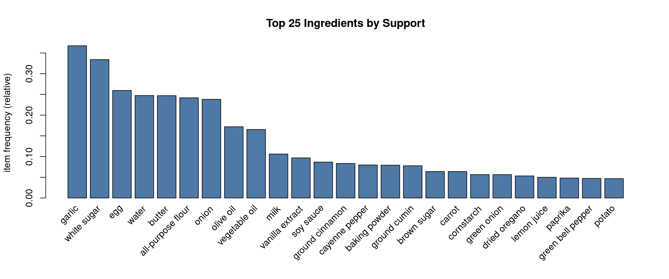
recipe_rules

#> set of 43 rules

# Top rules by lift
inspect(head(sort(recipe_rules, by = "lift"), n = 10))

#>      lhs                                         rhs                 support   
#> [1]  {baking powder}                          => {all-purpose flour} 0.06302132
#> [2]  {egg, butter, white sugar}               => {all-purpose flour} 0.05746061
#> [3]  {egg, butter}                            => {all-purpose flour} 0.07970343
#> [4]  {butter, white sugar}                    => {all-purpose flour} 0.07970343
#> [5]  {egg, white sugar}                       => {all-purpose flour} 0.08989805
#> [6]  {all-purpose flour, butter, white sugar} => {egg}               0.05746061
#> [7]  {baking powder}                          => {egg}               0.05468026
#> [8]  {all-purpose flour, white sugar}         => {egg}               0.08989805
#> [9]  {all-purpose flour, egg, white sugar}    => {butter}            0.05746061
#> [10] {milk}                                   => {egg}               0.07043559
#>      confidence coverage   lift     count
#> [1]  0.7953216  0.07924004 3.287939 136  
#> [2]  0.7750000  0.07414272 3.203927 124  
#> [3]  0.7136929  0.11167748 2.950478 172  
#> [4]  0.6935484  0.11492122 2.867198 172  
#> [5]  0.6783217  0.13253012 2.804249 194  
#> [6]  0.7209302  0.07970343 2.778156 124  
#> [7]  0.6900585  0.07924004 2.659190 118  
#> [8]  0.6759582  0.13299351 2.604853 194  
#> [9]  0.6391753  0.08989805 2.587880 124  
#> [10] 0.6637555  0.10611677 2.557829 152

Filtering Rules by Ingredient

# What goes with garlic?
garlic_rules <- subset(recipe_rules, subset = lhs %in% "garlic" & lift > 1.2)
inspect(head(sort(garlic_rules, by = "confidence"), n = 10))

#>     lhs                    rhs     support    confidence coverage  lift    
#> [1] {olive oil, garlic} => {onion} 0.05143652 0.4723404  0.1088971 1.983095
#>     count
#> [1] 111

Widget 4: Rule Explorer

Explore all mined recipe rules interactively. Brush the scatterplot, adjust thresholds, or search for specific ingredients.

import { ruleExplorerWidget } from "./widgets/association-rules/rule-explorer-widget.js"
viewof ruleExplorer = ruleExplorerWidget(transpose(rules_data))

Where Does Association Rule Mining Fit?

Association rules share ideas with many techniques you already know:

Direct Connections

Conditional Probability (STAT courses)

\[\text{confidence}(A \Rightarrow B) = P(B \mid A)\]

Confidence is conditional probability, estimated from data.

. . .

Bayesian Reasoning

\[\text{lift}(A \Rightarrow B) = \frac{P(B \mid A)}{P(B)}\]

Lift measures how much A changes our belief about B — like a likelihood ratio.

Unsupervised Discovery Family

Clustering (Week 10)

• Both discover structure without labels
• Clustering groups observations (rows)
• Association rules group items (columns)

Decision Trees (Week 9)

• Both produce interpretable IF→THEN rules
• Trees partition the feature space
• Association rules find co-occurrence patterns

Collaborative Filtering: The Famous Application

“Customers who bought X also bought Y”

This is literally association rule mining applied to recommendation systems.

Market Basket → Recommendations

Market Basket	Recommendation
Transaction = shopping cart	Transaction = user purchase history
Item = product	Item = product
Rule: {A} → {B}	Recommendation: “You might also like B”
High lift = genuine association	High lift = personalised recommendation

Key difference

Association rules find rules from all transactions together.

Modern recommender systems (Netflix, Spotify) use more sophisticated collaborative filtering (matrix factorisation, deep learning), but the core intuition is the same:

Find patterns of co-occurrence across many users/transactions.

Widget 5: Technique Comparison

Click any cell to expand the explanation. See how association rules compare with other methods you’ve learned.

import { techniqueComparisonWidget } from "./widgets/association-rules/technique-comparison-widget.js"
viewof techComparison = techniqueComparisonWidget()

Practical Tips

When to Use Association Rules

✅ Transactional data (baskets, carts, records)

✅ Binary/categorical variables

✅ Exploratory discovery — “what goes with what?”

✅ Large number of items with sparse transactions

✅ Business applications: cross-selling, layout optimisation, recommendations

When NOT to Use

❌ Small datasets (< 100 transactions) — rules will be unreliable

❌ Continuous data without discretisation

❌ When you need causal claims (rules show co-occurrence, not causation)

❌ When you have a specific target variable (use classification instead)

❌ Very dense data (every item in every transaction)

Practical Tips (Continued)

Choosing Thresholds

Parameter	Too low	Too high
min support	Millions of rules, most rare & unreliable	Only obvious, uninteresting patterns
min confidence	Many weak associations	Miss rules where consequent is rare

Start with support ≥ 0.01, confidence ≥ 0.5, then adjust based on domain knowledge and the number of rules produced.

Summary

Key Takeaways

1. Association rules discover co-occurrence patterns in transactional data
2. Support = how common, Confidence = how reliable, Lift = how interesting
3. High confidence alone is misleading — always check lift
4. Apriori prunes the search space using the antimonotone property
5. Association rules are the foundation of recommendation systems
6. Related to conditional probability, Bayes, clustering, and decision trees

Coming Up: Lab 11

In the lab you’ll practice with:

• The built-in Groceries dataset (9,835 transactions)
• The bank-rules.csv dataset (banking service cross-selling)
• Mining, inspecting, and filtering rules
• Using inspectDT() for interactive exploration

Study Guide

Chapter 8 of the course notes covers the same concepts with different examples and more mathematical detail.