161762 Multivariate Analysis for Big Data
Lecture 10: Cluster Analysis
Sergio Sclovich
Massey University
Fall 2026
Learning objectives
- Understand the basics of Cluster Analysis.
- Understand Hierarchical clustering.
Refresher Distance Matrix
\[
\mathbf{X}_{n \times p}
=
\begin{bmatrix}
x_{11} & \cdots & x_{1p} \\
\vdots & \ddots & \vdots \\
x_{n1} & \cdots & x_{np}
\end{bmatrix}
\Longrightarrow
\mathbf{D} =
\begin{bmatrix}
0 & d(x_1, x_2) & d(x_1, x_3) & \cdots & d(x_1, x_n) \\
d(x_2, x_1) & 0 & d(x_2, x_3) & \cdots & d(x_2, x_n) \\
d(x_3, x_1) & d(x_3, x_2) & 0 & \cdots & d(x_3, x_n) \\
\vdots & \vdots & \vdots & \ddots & \vdots \\
d(x_n, x_1) & d(x_n, x_2) & d(x_n, x_3) & \cdots & 0
\end{bmatrix}
\]
Fill \(d(x_n,x_n)\) with your favorite distance method.
Choose your analysis: ordination or Clustering.
Can we group units by being similar enough?
Clustering techniques intend to make groups out of the data.
Some applications are:
- Create groups when needed.
- Reduce data.
For example:
- Delineate market segments.
- Symptoms groups for diagnosis.
- Classify species.
Can we group units by being similar enough?
The aim of cluster analysis is to delineate “natural groups” of data, with high within-class similarity and low between-class similarity.
BUT this does not mean that the clusters actually exist!
Cluster Analysis will ALWAYS provide clusters (whether they exist or not).
Cluster profiling
Cluster profiling involves labelling a proposed cluster solution.
The objective is to identify the features, or combination of features, that uniquely describe each cluster.
It is useful to visualize clusters using an ordination, such as multidimensional scaling (MDS, which is also distance-based) or PCA.
can be achieved by various algorithms that differ significantly in their understanding of what constitutes a cluster.
If the clusters are well-separated, almost any clustering method performs well.
The process
\[
\mathbf{X}_{n \times p}
=
\begin{bmatrix}
x_{11} & \cdots & x_{1p} \\
\vdots & \ddots & \vdots \\
x_{n1} & \cdots & x_{np}
\end{bmatrix}
\Longrightarrow
\mathbf{D} =
\begin{bmatrix}
0 & d(x_1, x_2) & d(x_1, x_3) & \cdots & d(x_1, x_n) \\
d(x_2, x_1) & 0 & d(x_2, x_3) & \cdots & d(x_2, x_n) \\
d(x_3, x_1) & d(x_3, x_2) & 0 & \cdots & d(x_3, x_n) \\
\vdots & \vdots & \vdots & \ddots & \vdots \\
d(x_n, x_1) & d(x_n, x_2) & d(x_n, x_3) & \cdots & 0
\end{bmatrix}
\Longrightarrow
\mathbf{C} =
\begin{bmatrix}
C_1 \\ C_2 \\ \vdots \\ C_n \\
\end{bmatrix}
\]
Types of clustering methods
Hierarchical clustering: these algorithms form clusters by connecting objects based on their distance. A cluster can be understood in terms of the maximum distance required to connect its elements.
Centroid based clustering: each cluster is represented by a central vector, which is not necessarily a member of the data set. The number of clusters is pre defined (k) and the algorithm assigns the objects to the nearest cluster center.
Model-based clustering: This approach models the data as arising from a mixture of probability distributions.
Density-based clustering: clusters are defined as areas of higher density than the remainder of the data set.
Grid-based clustering: clusters are created by classfing cells of an arbitrary grid into clusters based on desnsity of points in each cell.
Hierarchical clustering
Hierarchy: an arrangement of items (objects, names, values, categories, etc.) that are represented as being “above”, “below”, or “at the same level as” one another.
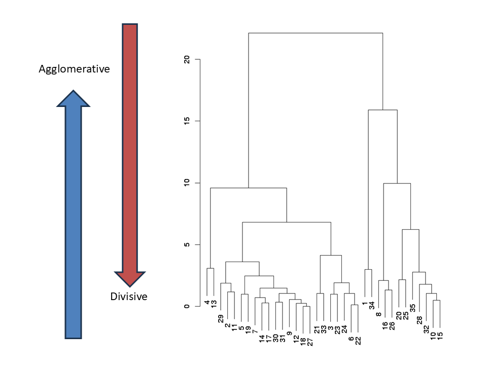
Agglomerative (bottom-up):begins with each data point as an individual cluster. Iteratevely, at each step, the algorithm merges the two most similar clusters based on a chosen distance metric and linkage criterion. This process continues until all data points are combined into a single cluster or a stopping criterion is met.
Divisive (top-down): starts with all data points in a single cluster and recursively splits the cluster into smaller ones. At each step, the algorithm selects a cluster and divides it into two or more subsets.
Hierarchical clustering:linkage criterion
A dendogram is a branching diagram that represents the relationships of similarity among a group of entities.
![]()
Hierarchical clustering: linkage criterion
As soon as you have a group, you’re dealing with more than one dissimilarity.
There are a number of ways to calculate an overall dissimilarity between groups of objects.
Some examples of linkage criterion are:
Nearest neighbour (single linkage): two objects or clusters fuse when their closest objects reach the similarity of the considered partition.
Complete linkage: two objects or clusters fuse when their most distant points reach the similarity of the considered partition.
Centroid linkage: the distance between clusters is the squared Euclidean distance between cluster centroids
Unweighted Pair-Group Method using Arithmetic averages (UPGMA): Two groups are joined with the highest average similarity between them (gives equal weights to original similarities).
Weighted Pair-Group Method using Arithmetic averages(WPGMA): Same as UPGMA, but gives equal weights to the branches of the dendrogram, rather than to the original similarities (e.g. for unequal sample sizes).
Ward’s minimum variance: finds the pair of objects or clusters whose fusion increases as little as possible the sum of the squared distances between objects and cluster centroids.
Agglomerative hierarchical clustering with nearest neighbour example
Grouping Customers by Product sales
\[
\begin{array}{c|cccccc}
& P1 & P2 & P3 & P4 & P5 & P6 \\
\hline
C1 & 9.7 & 21 & 19.4 & 7.7 & 32 & 36.5 \\
C2 & 8.1 & 16.7 & 18.3 & 7 & 30.3 & 32.9 \\
C3 & 13.5 & 27.3 & 26.8 & 10.6 & 41.9 & 48.1 \\
C4 & 11.5 & 24.3 & 24.5 & 9.3 & 40 & 44.6 \\
C5 & 10.7 & 23.5 & 21.4 & 8.5 & 28.8 & 37.6 \\
C6 & 9.6 & 22.6 & 21.1 & 8.3 & 34.4 & 43.1 \\
C7 & 10.3 & 22.1 & 19.1 & 8.1 & 32.2 & 35
\end{array}
\Longrightarrow
\begin{array}{c|ccccccc}
& C1 & C2 & C3 & C4 & C5 & C6 & C7 \\
\hline
C1 & 0 & & & & & & \\
C2 & 1.91 & 0 & & & & & \\
C3 & 5.38 & 7.12 & 0 & & & & \\
C4 & 3.38 & 5.06 & 2.14 & 0 & & & \\
C5 & 1.51 & 3.19 & 4.57 & 2.91 & 0 & & \\
C6 & 1.56 & 3.18 & 4.21 & 2.20 & 1.67 & 0 & \\
C7 & 0.66 & 2.39 & 5.12 & 3.24 & 1.26 & 1.71 & 0
\end{array}
\]
Example
Agglomerative hierarchical clustering with nearest neighbour
\[
\tiny
\begin{array}{c|ccccccc}
& C1 & C2 & C3 & C4 & C5 & C6 & C7 \\
\hline
C1 & 0 & & & & & & \\
C2 & 1.91 & 0 & & & & & \\
C3 & 5.38 & 7.12 & 0 & & & & \\
C4 & 3.38 & 5.06 & 2.14 & 0 & & & \\
C5 & 1.51 & 3.19 & 4.57 & 2.91 & 0 & & \\
C6 & 1.56 & 3.18 & 4.21 & 2.20 & 1.67 & 0 & \\
C7 & \color{purple}{0.66} & 2.39 & 5.12 & 3.24 & 1.26 & 1.71 & 0
\end{array}
\]
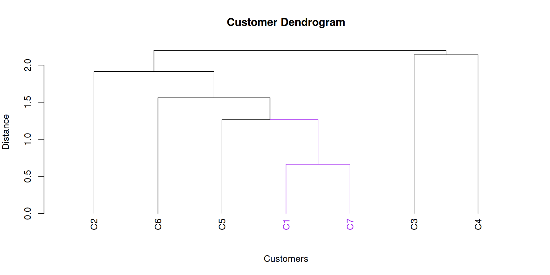
- Step 1: C1 joins C7 at a distance of 0.66
Example
Agglomerative hierarchical clustering with nearest neighbour
\[
\tiny
\begin{array}{c|ccccccc}
& C1 & C2 & C3 & C4 & C5 & C6 & C7 \\
\hline
C1 & 0 & & & & & & \\
C2 & 1.91 & 0 & & & & & \\
C3 & 5.38 & 7.12 & 0 & & & & \\
C4 & 3.38 & 5.06 & 2.14 & 0 & & & \\
C5 & 1.51 & 3.19 & 4.57 & 2.91 & 0 & & \\
C6 & 1.56 & 3.18 & 4.21 & 2.20 & 1.67 & 0 & \\
C7 & \color{purple}{0.66} & 2.39 & 5.12 & 3.24 & \color{red}{1.26} & 1.71 & 0
\end{array}
\]
Example
Agglomerative hierarchical clustering with nearest neighbour
\[
\tiny
\begin{array}{c|ccccccc}
& C1 & C2 & C3 & C4 & C5 & C6 & C7 \\
\hline
C1 & 0 & & & & & & \\
C2 & 1.91 & 0 & & & & & \\
C3 & 5.38 & 7.12 & 0 & & & & \\
C4 & 3.38 & 5.06 & 2.14 & 0 & & & \\
C5 & \color{green}{1.51} & 3.19 & 4.57 & 2.91 & 0 & & \\
C6 & \color{green}{1.56} & 3.18 & 4.21 & 2.20 & 1.67 & 0 & \\
C7 & \color{purple}{0.66} & 2.39 & 5.12 & 3.24 & \color{red}{1.26} & 1.71 & 0
\end{array}
\]
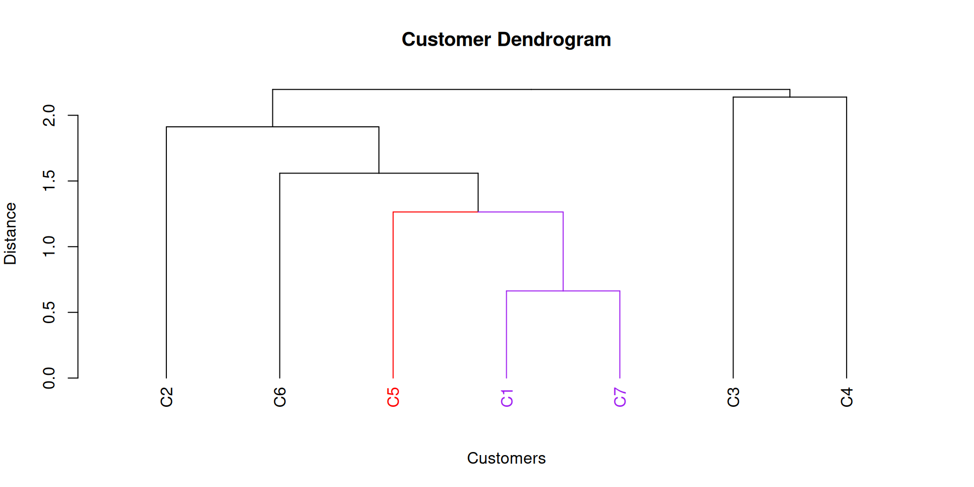
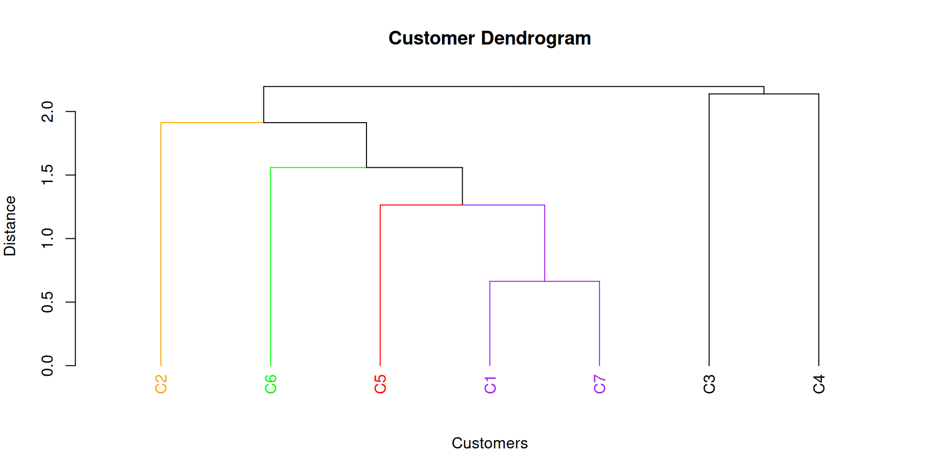
Step 1: C1 joins C7 at a distance of 0.66.
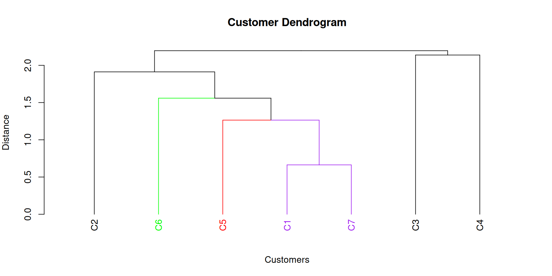
Step 2: C5 joins (C1,C7) at a distance of 1.26.
Step 3: (C6) joins (C1, C7, C5) at a distance of 1.56
Example
Agglomerative hierarchical clustering with nearest neighbour
\[
\tiny
\begin{array}{c|ccccccc}
& C1 & C2 & C3 & C4 & C5 & C6 & C7 \\
\hline
C1 & 0 & & & & & & \\
C2 & \color{orange}{1.91} & 0 & & & & & \\
C3 & 5.38 & 7.12 & 0 & & & & \\
C4 & 3.38 & 5.06 & 2.14 & 0 & & & \\
C5 & \color{green}{1.51} & 3.19 & 4.57 & 2.91 & 0 & & \\
C6 & \color{green}{1.56} & 3.18 & 4.21 & 2.20 & \color{orange}{1.67} & 0 & \\
C7 & \color{purple}{0.66} & 2.39 & 5.12 & 3.24 & \color{red}{1.26} & \color{orange}{1.71} & 0
\end{array}
\]
Step 1: C1 joins C7 at a distance of 0.66.
Step 2: C5 joins (C1,C7) at a distance of 1.26.
Step 3: (C6) joins (C1, C7, C5) at a distance of 1.56.
Step 4: (C2) joins (C1, 5, 6, 7) at a distance of 1.91.
Example
Agglomerative hierarchical clustering with nearest neighbour
\[
\tiny
\begin{array}{c|ccccccc}
& C1 & C2 & C3 & C4 & C5 & C6 & C7 \\
\hline
C1 & 0 & & & & & & \\
C2 & \color{orange}{1.91} & 0 & & & & & \\
C3 & 5.38 & 7.12 & 0 & & & & \\
C4 & 3.38 & 5.06 & \color{blue}{2.14} & 0 & & & \\
C5 & \color{green}{1.51} & 3.19 & 4.57 & 2.91 & 0 & & \\
C6 & \color{green}{1.56} & 3.18 & 4.21 & 2.20 & \color{orange}{1.67} & 0 & \\
C7 & \color{purple}{0.66} & 2.39 & 5.12 & 3.24 & \color{red}{1.26} & \color{orange}{1.71} & 0
\end{array}
\]
Step 1: C1 joins C7 at a distance of 0.66.
Step 2: C5 joins (C1,C7) at a distance of 1.26.
Step 3: (C6) joins (C1, C7, C5) at a distance of 1.56.
Step 4: (C2) joins (C1, 5, 6, 7) at a distance of 1.91.
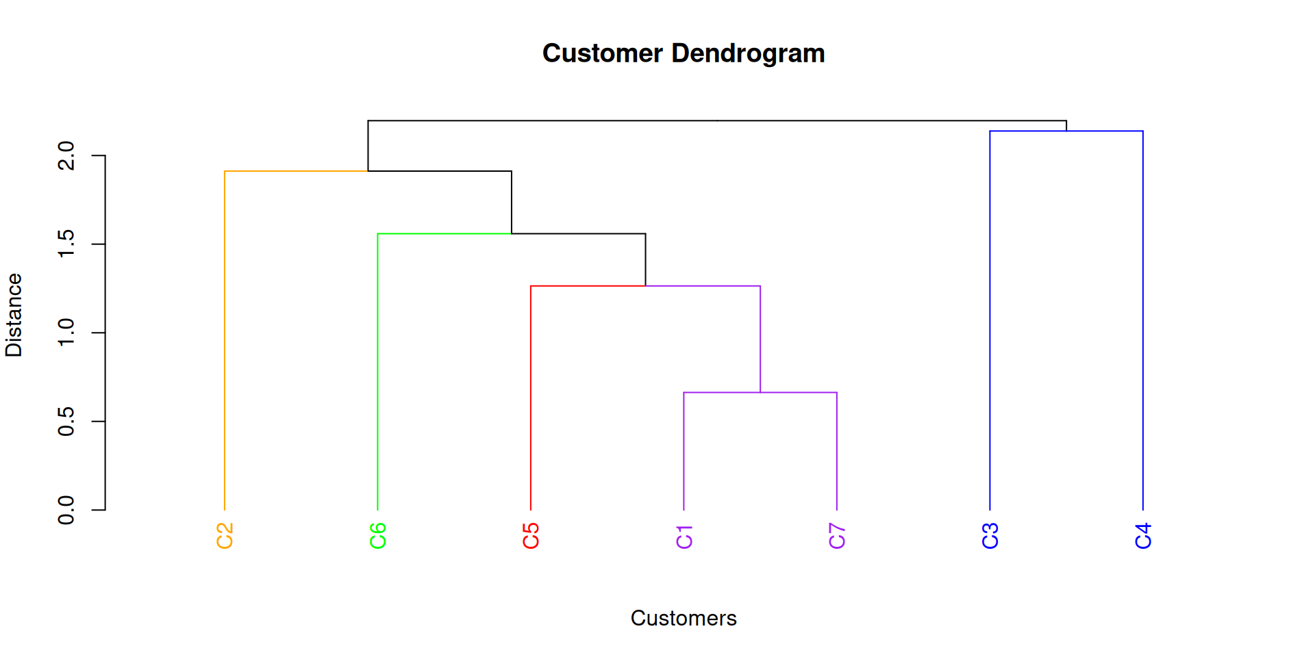
Step 5: (C3) joins (C4) at a distance of 2.14.
Example
Agglomerative hierarchical clustering with nearest neighbour
\[
\tiny
\begin{array}{c|ccccccc}
& C1 & C2 & C3 & C4 & C5 & C6 & C7 \\
\hline
C1 & 0 & & & & & & \\
C2 & \color{orange}{1.91} & 0 & & & & & \\
C3 & 5.38 & 7.12 & 0 & & & & \\
C4 & 3.38 & 5.06 & \color{blue}{2.14} & 0 & & & \\
C5 & \color{green}{1.51} & 3.19 & 4.57 & 2.91 & 0 & & \\
C6 & \color{green}{1.56} & 3.18 & 4.21 & 2.20 & \color{orange}{1.67} & 0 & \\
C7 & \color{purple}{0.66} & 2.39 & 5.12 & 3.24 & \color{red}{1.26} & \color{orange}{1.71} & 0
\end{array}
\]
Step 1: C1 joins C7 at a distance of 0.66.
Step 2: C5 joins (C1,C7) at a distance of 1.26.
Step 3: (C6) joins (C1, C7, C5) at a distance of 1.56.
Step 4: (C2) joins (C1, 5, 6, 7) at a distance of 1.91.
Step 5: (C3) joins (C4) at a distance of 2.14.
Step 6: (C3, 4) joins (C1, 5, 6, 7) at a distance of 2.20.
Considerations about hierarchical clustering
- Strengths
- Intuitive.
- Dendrogram highlights relationships between groups.
- Don‘t have to choose 𝑘 a priori. Can cut the tree at any level.
- Weaknesses
- Can be infeasible for very large datasets.
- Results dependent on particular algorithm used.
- Not easy to assign new cases.
General considerations about cluster analysis
Problems occur when the data are actually along a continuum (e.g., along a gradient, where no natural “boundaries” exist).
Arbitrary decision must be made about where to “draw the line” across a dendrogram.
Clustering procedures will find groups even when there are none (i.e., in random data).
Groups obtained from a cluster analysis may or may not be “real”.