161762 Multivariate Analysis for Big Data
Lecture 3: Introduction to Principal Components Analysis
Sergio Sclovich
Massey University
Fall 2026
Learning objectives
Explain basic concepts of Principal Components Analysis (PCA).
Explain eigenvalue decomposition and some properties of eigenvalues.
Understand strategies to reduce dimensionality.
How do we reduce the number of dimensions?
A typical dataset is a matrix:
Rows: sample units (customers, patients, devices)
Columns: variables (products, biomarkers, measurements)
Example:
| Customer | Product 1 | Product 2 | Product 3 | Churn |
|---|---|---|---|---|
| 1 | 5 | 6 | 1 | 0 |
| 2 | 3 | 5 | 1 | 0 |
| 3 | 3 | 6 | 2 | 0 |
| 4 | 3 | 8 | 4 | 0 |
Each variable is a dimension.
How do we reduce the number of dimensions?
How do we reduce the number of dimensions?
How do we reduce the number of dimensions?
How do we reduce the number of dimensions?
We just performed a Principal components analysis (PCA)
Is a dimension reduction method that creates variables called principal components (Eigenvectors).
It creates as many components as there are input variables.
X (n × p)
↓
Covariance matrix Σ (p × p)
↓
Eigenvectors / eigenvalues
↓
Principal components
Eigenvalue decomposition
Data Matrix
\[ \mathbf{X}_{n \times p} = \begin{bmatrix} x_{11} & \cdots & x_{1p} \\ \vdots & \ddots & \vdots \\ x_{n1} & \cdots & x_{np} \end{bmatrix} \]
\[ \Longrightarrow \]
Variance–Covariance Matrix
\[ \boldsymbol{S} = \begin{bmatrix} \color{red}{\mathrm{Var}(X_1)} & \mathrm{Cov}(X_1,X_2) & \cdots & \mathrm{Cov}(X_1,X_p) \\ \mathrm{Cov}(X_2,X_1) & \color{red}{\mathrm{Var}(X_2)} & \cdots & \mathrm{Cov}(X_2,X_p) \\ \vdots & \vdots & \ddots & \vdots \\ \mathrm{Cov}(X_p,X_1) & \mathrm{Cov}(X_p,X_2) & \cdots & \color{red}{\mathrm{Var}(X_p)} \end{bmatrix} \]
- Covariance captures shape.
- Variance captures spread.
\[ \Longrightarrow \]
Eigenanalysis Procedure
\[ \mathbf{S}\mathbf{v}_i = \lambda_i \mathbf{v}_i \qquad \Longrightarrow \qquad \mathbf{S} = \mathbf{V}\mathbf{\Lambda}\mathbf{V}^\top \]
where
\[ \mathbf{S}_{p \times p} \qquad \boldsymbol{\Lambda} = \begin{bmatrix} \lambda_1 & 0 & \cdots & 0 \\ 0 & \lambda_2 & \cdots & 0 \\ \vdots & \vdots & \ddots & \vdots \\ 0 & 0 & \cdots & \lambda_p \end{bmatrix} \qquad \mathbf{V} = \begin{bmatrix} v_1 & v_2 & \cdots & v_p \end{bmatrix} \]
some comments about eigenvectors and eigenvalues
The eigenvectors and eigenvalues represent the “axes” (and size) of the transformation.
There are as many eigenvectors and eigenvalues as dimensions in the original dataset.
The eigenvectors maximizes total variation along the axis.
The eigenvectors are orthogonal, hence independent.
eigenvalues can also be read as “Information explained by” or “variance accounted for” an eigenvector.
The eigenvectors are usually order by decreasing associated eigenvalue.
How do we reduce the number of dimensions?
If eigenvalues represent the information explained by the corresponding eigenvector.
And only the first ones have the highest values.
Why do I need all of them?
How do we reduce the number of dimensions?
We reduce the number of dimensions by selecting those eigenvectors that have the highest associated eigenvalues.
Selection of the number of dimensions
\[ \begin{array}{ll} \lambda_T = \lambda_1 + \lambda_2 + \dots + \lambda_i & \rightarrow \quad \text{Overall variance} \\[8pt] \lambda_i \; (\text{proportion}) = \dfrac{\lambda_i}{\lambda_T} & \\[8pt] \text{Cumulative } \Lambda = \dfrac{\sum \lambda_{\text{interest}}}{\lambda_T} & \end{array} \]
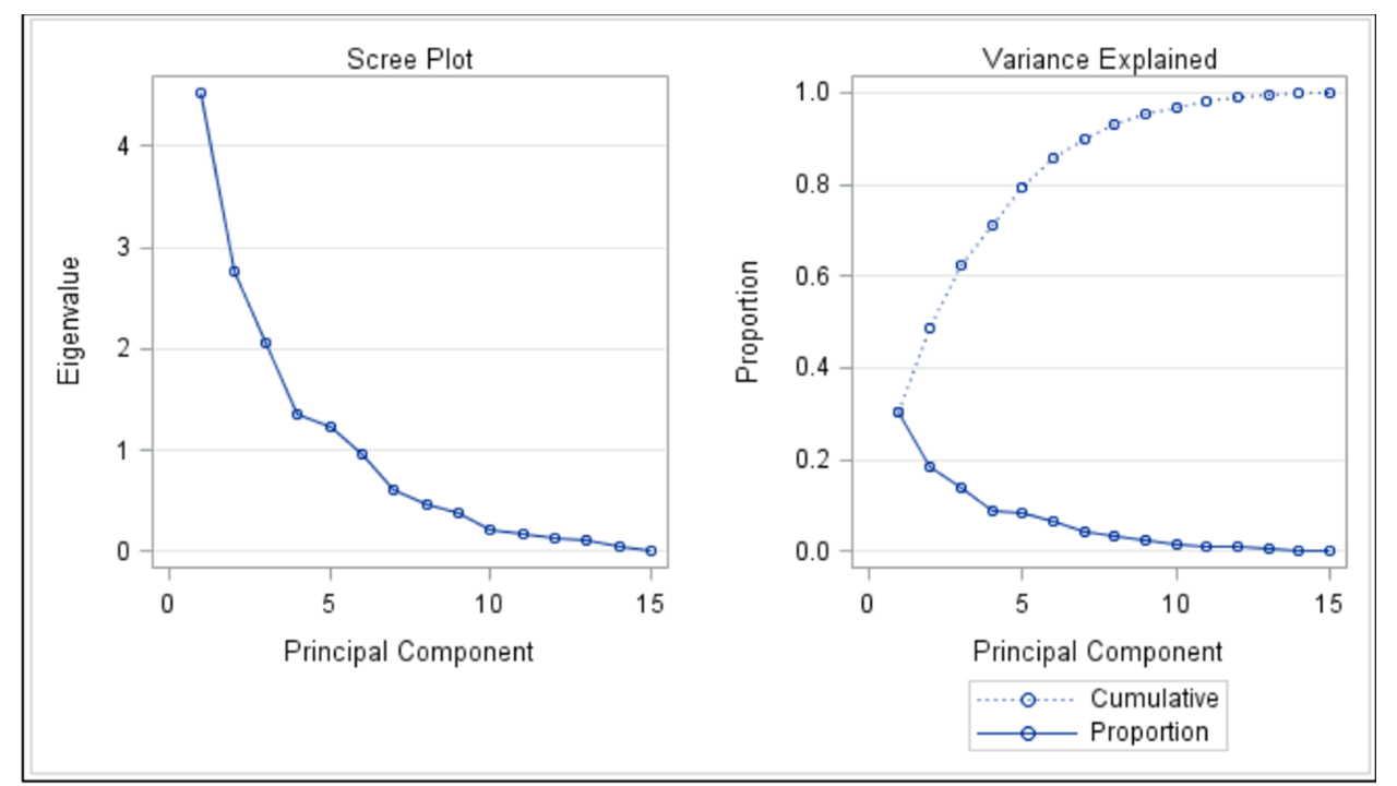
Selection of the number of dimensions
Screeplot