161762 Multivariate Analysis for Big Data
Lecture 5: Distance methods
Massey University
Fall 2026
Learning objectives
Define the concept of distance.
Understand the basics of a distance method.
Recognize different types of distances and assess the right use for each type.
What is a Distance?
We can quantify the distance between any pair of sampling units to build a Distance Matrix.
This is a useful starting point for some multivariate analyses.
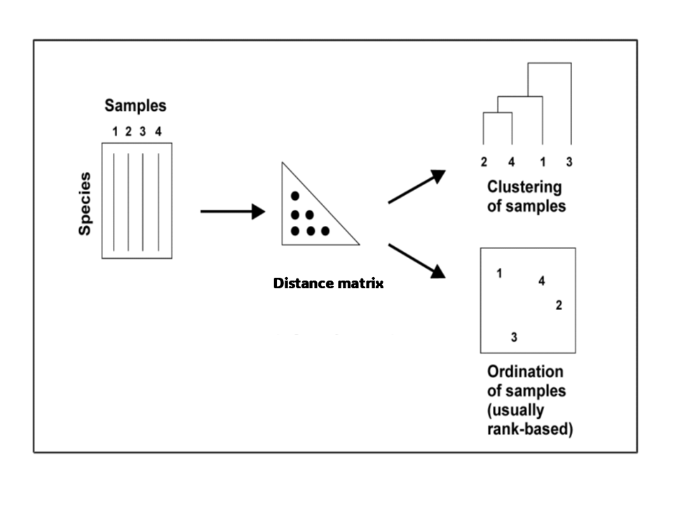
What is a Distance?
With a Var-Covar Matrix I can capture the relationships among variables.
With a Distance Matrix I can capture the relationships among individuals.
\[ \mathbf{X}_{n \times p} = \begin{bmatrix} x_{11} & \cdots & x_{1p} \\ \vdots & \ddots & \vdots \\ x_{n1} & \cdots & x_{np} \end{bmatrix} \Longrightarrow \mathbf{D} = \begin{bmatrix} 0 & d(x_1, x_2) & d(x_1, x_3) & \cdots & d(x_1, x_n) \\ d(x_2, x_1) & 0 & d(x_2, x_3) & \cdots & d(x_2, x_n) \\ d(x_3, x_1) & d(x_3, x_2) & 0 & \cdots & d(x_3, x_n) \\ \vdots & \vdots & \vdots & \ddots & \vdots \\ d(x_n, x_1) & d(x_n, x_2) & d(x_n, x_3) & \cdots & 0 \end{bmatrix} \]
- Another way of thinking of a distance is thinking about similarity (or disimilarity).
What is similarity?

What is similarity?
The answer to this question largely depends on how you choose to operationalize (define) similarity.
Depending on the context it could have different names.
- Measures of association.
- coefficients or indices of resemblance.
- Similarity or dissimilarity measures.
- Distance measures.
Different types of similarities/dissimilarities.
Euclidean.
Manhattan
Mahalanobis
Bray-Curtis
Sokal and Sneath
Rogers and Tanimoto
Yule coefficient
Pearson’s Phi
Sorensen’s coefficient
Russell and Rao
Kulczynski
Ochiai
Faith distance
Euclidean Distance
Is a standard distance from one point to another “as the crow flies”.
\[ d_{ij} = \sqrt{ \sum_{k=1}^{p} \underbrace{(y_{ik} - y_{jk})^2}_{\text{difference on variable } k} } \\[4em] \begin{aligned} d_{ij} &: \text{distance between samples } i \text{ and } j \\ y_{ik} &: \text{value of variable } k \text{ for sample } i \\ y_{jk} &: \text{value of variable } k \text{ for sample } j \end{aligned} \]
Euclidean Distance
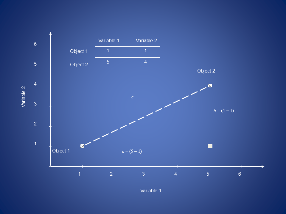
\[c = \sqrt{a^2 + b^2}\]
\[d_{1,2} = \sqrt{(y_{1,1} - y_{2,1})^2 + (y_{1,2} - y_{2,2})^2}\]
\[d_{1,2} = \sqrt{(5-1)^2 + (4-1)^2} = 5\]
In PCA the new orthogonal basis preserves the squared Euclidean distances between points as much as possible in the reduced-dimensional space.
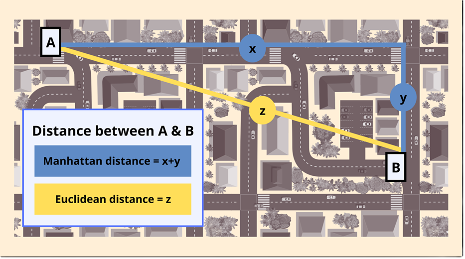
Manhattan Distance (Taxicab)
\[
d_{ij} = \sum_{k=1}^{p}
\underbrace{\left| y_{ik} - y_{jk} \right|}_{\text{absolute difference on variable } k}
\quad
\text{Less sensible to outliers than Euclidean
}
\] 
We can measure similarity with qualitative variables
Binary variables
Let’s say we have to customers x and y. Also we have the data fo what products they bought.
| Customer | P1 | P2 | P3 | P4 |
|---|---|---|---|---|
| X | 1 | 1 | 0 | 0 |
| Y | 1 | 0 | 1 | 0 |
we will consider the following notations
- a represents the count of times we have 1 for both cases.
- b represents the count of times we have 0 for customer y and 1 for customer x.
- c represents the count of times we have 1 for customer y and 0 for customer x.
- d represents the count of times we have 0 for both customers.
Contingency table
| 1 | 0 | |
|---|---|---|
| 1 | a | b |
| 0 | c | d |
Binary variables
| Customer | P1 | P2 | P3 | P4 | P5 | P6 |
|---|---|---|---|---|---|---|
| X | 1 | 1 | 0 | 0 | 1 | 0 |
| Y | 1 | 0 | 1 | 0 | 1 | 1 |
Contingency table
| 1 | 0 | |
|---|---|---|
| 1 | a | b |
| 0 | c | d |
Binary variables
| Customer | P1 | P2 | P3 | P4 | P5 | P6 |
|---|---|---|---|---|---|---|
| X | 1 | 1 | 0 | 0 | 1 | 0 |
| Y | 1 | 0 | 1 | 0 | 1 | 1 |
Contingency table
| 1 | 0 | |
|---|---|---|
| 1 | 2 | b |
| 0 | c | d |
Binary variables
| Customer | P1 | P2 | P3 | P4 | P5 | P6 |
|---|---|---|---|---|---|---|
| X | 1 | 1 | 0 | 0 | 1 | 0 |
| Y | 1 | 0 | 1 | 0 | 1 | 1 |
Contingency table
| 1 | 0 | |
|---|---|---|
| 1 | 2 | 1 |
| 0 | c | d |
Binary variables
| Customer | P1 | P2 | P3 | P4 | P5 | P6 |
|---|---|---|---|---|---|---|
| X | 1 | 1 | 0 | 0 | 1 | 0 |
| Y | 1 | 0 | 1 | 0 | 1 | 1 |
Contingency table
| 1 | 0 | |
|---|---|---|
| 1 | 2 | 1 |
| 0 | 2 | d |
Binary variables
| Customer | P1 | P2 | P3 | P4 | P5 | P6 |
|---|---|---|---|---|---|---|
| X | 1 | 1 | 0 | 0 | 1 | 0 |
| Y | 1 | 0 | 1 | 0 | 1 | 1 |
Contingency table
| 1 | 0 | |
|---|---|---|
| 1 | 2 | 1 |
| 0 | 2 | 1 |
Now let’s measure some qualitative distance
###Euclidian distance
\[ d_{xy} = \sqrt{b^2+c^2} \]
- Euclidean distance has min zero and no max.
- It reflects dissimilarity.
Simple matching
\[ d_{xy} = \dfrac{a+d}{a+b+c+d} \]
- Simple matching limits between 0 and 1.
- In this case, dissimilarity is (1 – similarity)
We can expand now to other qualitative variables
Nominal — categorical data with no natural order (e.g. colour, gender, ethnicity).
Ordinal — categorical data with a meaningful order, but unequal intervals between values (e.g. low/medium/high, survey ratings).
We can use Simple matching for this type of variables
\[d_(xy) = \frac{1}{n} \sum_{i=1}^{n} \mathbb{1}(x_i = y_)\]
or you can consider de opposite for dissimilarity
\[d_(xy) = \frac{1}{n} \sum_{i=1}^{n} \mathbb{1}(x_i \neq y_)\]
Distance measures for mixed data
What if data has both categorical & numeric variables and you wish to use them both?
| Customer | Age | Income ($k) | Segment | Has App | Satisfaction |
|---|---|---|---|---|---|
| A | 25 | 40 | Retail | Yes | Low |
| B | 45 | 80 | Corporate | No | Medium |
| C | 35 | 60 | Retail | Yes | High |
| D | 50 | 90 | Corporate | No | Medium |
What type of variable are each of these?
- Numeric
- Age
- Income
- Categorical (nominal)
- Segment
- Binary
- Has App
- Ordinal
- Satisfaction (Low < Medium < High)
Gower’s distance
Gower Distance
\[ d_{ij} = \frac{\sum_{k=1}^{p} w_k \, d_{ijk}}{\sum_{k=1}^{p} w_k } \qquad d_{ijk} = \begin{cases} 1 - \frac{|x_{ik} - x_{jk}|}{R_k}, & \text{numeric} \\ 1, & x_{ik} = x_{jk} \ (\text{categorical}) \\ 0, & x_{ik} \ne x_{jk} \ (\text{categorical}) \end{cases} \\[3em] \begin{aligned} d_{ij} &: \text{distance between observations } i,j \\ w_k &: \text{variable weight} \\ d_{ijk} &: \text{partial distance} \\ R_k &: \text{range of variable } k \end{aligned} \]
- Rescale numeric variables so their range is [0,1].
- Recode nominal variables with >2 levels into multiple binary variables.
- Rescale ordinal variables (Podani’s method, and others).
- Calculate the similarity of each variable and average to get a total similarity.
- Calculate D = 1 – G.
Jaccard similarity
Are two objects more similar because they both lack some particular characters?
- If 1 and 0 are equally important is a symmetric binary variable.
- If 1 is more important than 0 is an asymmetric Binary variable.
\[ S_{ij}=\frac{a}{a+b+c} \]
symetric vs asymetric binary variables
| Customer | P1 | P2 | P3 | P4 | P5 | P6 |
|---|---|---|---|---|---|---|
| X | 1 | 1 | 0 | 0 | 1 | 0 |
| Y | 1 | 0 | 1 | 0 | 1 | 1 |
| 1 | 0 | |
|---|---|---|
| 1 | 2 | 1 |
| 0 | 2 | 1 |
\[ \text{Simple mistmatch} = \frac{2+1}{2+1+2+1} = 0.5 \\[1em] \text{Jaccard} = \frac{2}{2+1+2} = 0.4 \]