161762 Multivariate Analysis for Big Data

Learning objectives

Understand the basics of Multidimensional Scaling.
Understand the basics of Factor Analysis.

Refresher Distance Matrix

\[ \mathbf{X}_{n \times p} = \begin{bmatrix} x_{11} & \cdots & x_{1p} \\ \vdots & \ddots & \vdots \\ x_{n1} & \cdots & x_{np} \end{bmatrix} \Longrightarrow \mathbf{D} = \begin{bmatrix} 0 & d(x_1, x_2) & d(x_1, x_3) & \cdots & d(x_1, x_n) \\ d(x_2, x_1) & 0 & d(x_2, x_3) & \cdots & d(x_2, x_n) \\ d(x_3, x_1) & d(x_3, x_2) & 0 & \cdots & d(x_3, x_n) \\ \vdots & \vdots & \vdots & \ddots & \vdots \\ d(x_n, x_1) & d(x_n, x_2) & d(x_n, x_3) & \cdots & 0 \end{bmatrix} \]

Fill \(d(x_n,x_n)\) with your favorite distance method.
Choose your analysis: ordination or Clustering (later in the ocurse)

Multidimensional Scaling (MDS)

MDS & Related Methods - Historical Timeline

1952 | Torgerson introduces Metric MDS
1964 | Kruskal develops Non-metric MDS
1966 | Gower formalizes Classical MDS as Principal Coordinates Analysis (PCoA)
1971 | Gower publishes the Gower Similarity Coefficient (handles mixed data types)

Multidimensional Scaling (MDS)

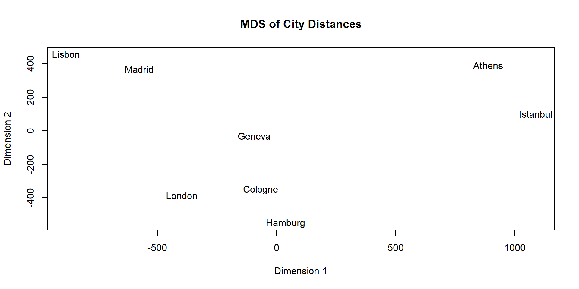
Ordinate your samples in a reduce dimensional space.
MDS is an unconstrained ordination method.

Multidimensional Scaling (MDS)

	Athens	Cologne	Geneva	Hamburg	Istanbul	Lisbon	London	Madrid
Athens	0
Cologne	1212	0
Geneva	1068	323	0
Hamburg	1268	227	540	0
Istanbul	345	1239	1190	1236	0
Lisbon	1772	1149	929	1366	2003	0
London	1501	331	468	463	1562	972	0
Madrid	1466	883	627	1107	1686	319	774	0

Multidimensional Scaling (MDS)

Original

	Ath	Col	Gen	Ham	Ist	Lis	Lon	Mad
Ath	0
Col	1212	0
Gen	1068	323	0
Ham	1268	227	540	0
Ist	345	1239	1190	1236	0
Lis	1772	1149	929	1366	2003	0
Lon	1501	331	468	463	1562	972	0
Mad	1466	883	627	1107	1686	319	774	0

MDS

	Ath	Col	Gen	Ham	Ist	Lis	Lon	Mad
Ath	0
Col	1211	0
Gen	1069	324	0
Ham	1269	225	538	0
Ist	352	1241	1189	1236	0
Lis	1773	1149	927	1366	2003	0
Lon	1502	331	467	466	1563	973	0
Mad	1466	883	626	1107	1687	318	775	0

Adequacy of the ordination

PCA
- Euclidean distances in the ordination vs. Euclidean distances among the points based on the full set of (standardized) original variables
MDS
- Euclidean distances in the ordination vs. original dissimilarities or distances (based on a chosen measure).

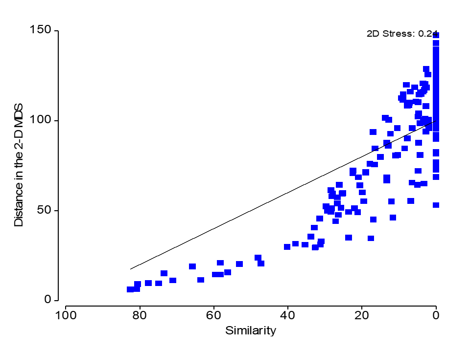
Stress

\[ \text{S} = \frac{ \overbrace{\displaystyle \sum_{j<k} \left( d_{jk} - \delta_{jk} \right)^2}^{\text{Sum of squared residuals (MDS distance vs perfect regression)}} }{ \underbrace{\displaystyle \sum_{j<k} \delta_{jk}^2}_{\text{Sum of squared perfect regression distances (original distances)}} } \]

Stress

Is a measure of how good the fit is between the original distances and the new distances on the plot.
The lower the stress, the more the MDS plot reflects real distance structures in the data.
A published MDS plot should always state a value for stress. (if done iteratively).
Rule of thumb:
- Stress < 0.1 Good.
- 0.1 < Stress < 0.2 OK
- Stress > 0.2 Not so good
- Stress > 0.3 No better than random!

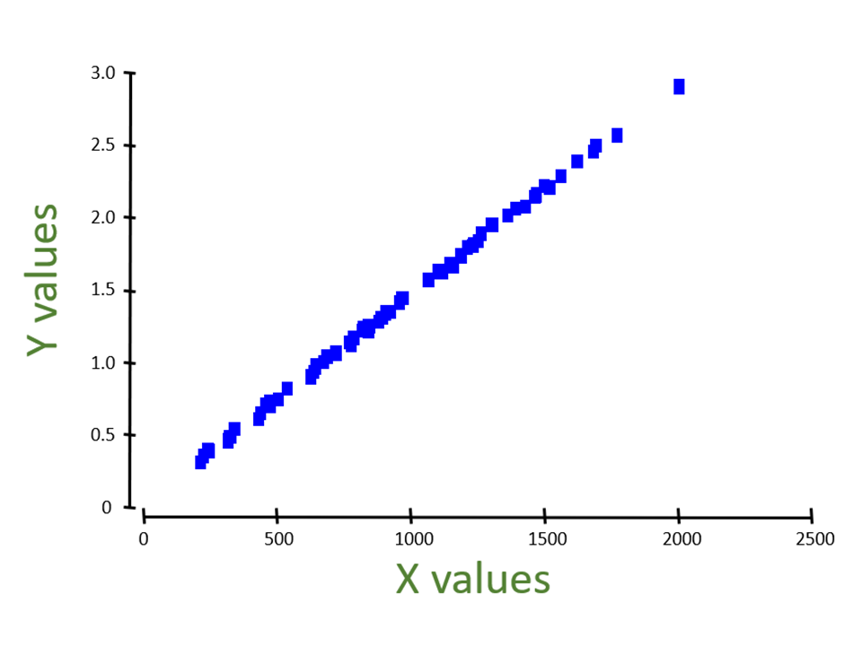
Metric VS Non-metric MDS (nMDS)

Metric MDS fits a strictly linear regression line (constant slope; fixed at the origin)

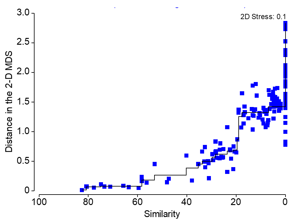
nMDS fits a monotonically increasing regression line (a step function)

Metric VS Non-metric MDS (nMDS)

In a nMDS, points are positioned according to their ranked distances.
Therefore, the specific values along the axes of a nMDS plot have no particular meaning – they are arbitrary.
nMDS is flexible. You can use any measure of distance, dissimilarity or similarity may be used as the basis of the analysis.
nMDS is generally more robust to outliers.
nMDS tends to be more computationally intense.

Considerations about MDS

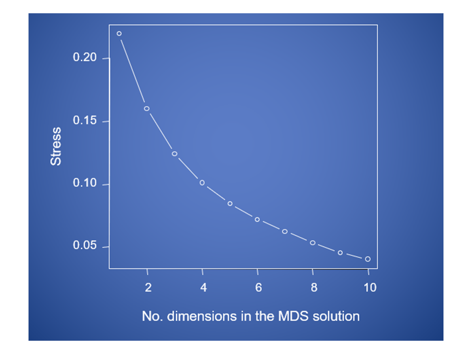
Stress will decrease with increasing numbers of MDS axes

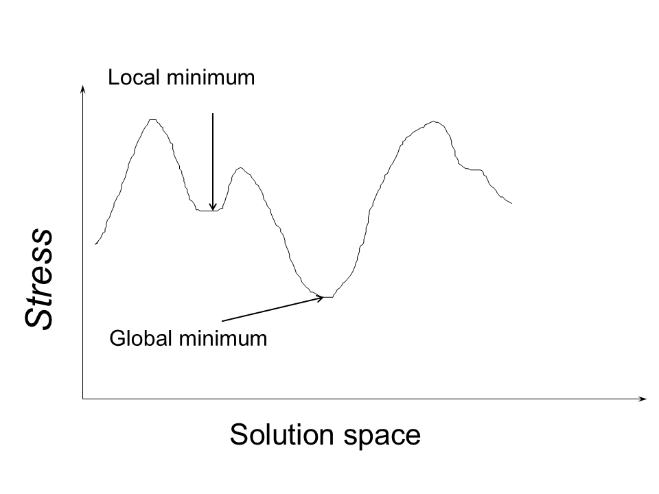
Considerations about MDS

The results space is dependent on the starting point.
Stress can fall into local minima.

Factor Analysis (FA)

Back to the var-covar (R) matrix.
In PCA, R is eigen decomposed.
In FA, R-U. where U is the unique part. R-U is known as Communality.

\[ \begin{bmatrix} 1 & r_{12} & \cdots & r_{1p} \\ r_{21} & 1 & \cdots & r_{2p} \\ \vdots & \vdots & \ddots & \vdots \\ r_{p1} & r_{p2} & \cdots & 1 \end{bmatrix} - \begin{bmatrix} u_1 & 0 & \cdots & 0 \\ 0 & u_2 & \cdots & 0 \\ \vdots & \vdots & \ddots & \vdots \\ 0 & 0 & \cdots & u_p \end{bmatrix} \]

FA analyzes only the common variance of the observed variables.

Factor Analysis (FA) considerations

Since the concept of common variance is hypothetical, we never know exactly in advance what percentage of variance is common and what proportion is unique among variables.
Factor scores are not linear combinations of the variables. They are estimates of latent factors. Try to avoid data fishing problems by doing the following:
1. Carefully selecting your manifest variables
2. Using rotation to interpret the factors
3. Performing a confirmatory factor analysis to test
  hypotheses about the adequacy of the factor solution