35 Regression with Autoregressive Errors
35.1 Regression with Autoregressive Errors
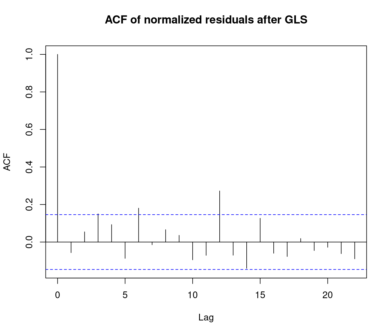
The previous lecture showed how to diagnose autocorrelation in regression residuals. This lecture keeps the same mean structure ideas, but changes the model for the errors.
By the end of this lecture, students should be able to:
- Write down a regression model with AR(1) errors.
- Explain why autocorrelated errors distort ordinary standard errors.
- Fit a regression model with
gls()andcorAR1(). - Check whether normalized residuals look closer to white noise.
35.2 Why Ordinary Least Squares Is Not Enough
If the residuals are autocorrelated, the ordinary least-squares coefficient estimates are often still unbiased, but their reported standard errors are usually too small. The main practical consequences are:
- test statistics are too large,
- p-values are too small,
- confidence intervals are too narrow.
So we keep the regression mean structure, but replace the independence assumption with a more realistic error process.
35.3 The AR(1) Error Model
A first-order autoregressive error model is \[\varepsilon_t = \phi \varepsilon_{t-1} + \eta_t,\] where \(\eta_t\) is white noise.
- If \(\phi > 0\), nearby errors tend to move in the same direction.
- If \(\phi < 0\), nearby errors tend to alternate.
- If \(\phi = 0\), we are back to independent errors.
More generally, the lag-\(k\) autocorrelation is \(\phi^k\), so the effect gradually dies away through time.
35.4 Main Worked Example: Tourism in Victoria
These data are monthly room nights occupied in hotels, motels, and guesthouses in Victoria from January 1980 to December 1994.
tourism <- read_csv("../data/motel.csv", show_col_types = FALSE) |>
    mutate(Date = as.Date(Date), Time = round(time_length(Date - min(Date), unit = "month")),
        Month = factor(month(Date, label = TRUE), ordered = FALSE), Year = year(Date))

tourism |>
    head() |>
kable()| Date | RoomNights | AvePrice | Time | Month | Year |
|---|---|---|---|---|---|
| 1980-01-01 | 276986 | 27.70 | 0 | Jan | 1980 |
| 1980-02-01 | 260633 | 28.67 | 1 | Feb | 1980 |
| 1980-03-01 | 291551 | 28.60 | 2 | Mar | 1980 |
| 1980-04-01 | 275383 | 28.34 | 3 | Apr | 1980 |
| 1980-05-01 | 275302 | 28.66 | 4 | May | 1980 |
| 1980-06-01 | 231693 | 28.57 | 5 | Jun | 1980 |
35.4.1 Ordinary Regression First
Analysis of Variance Table

Response: RoomNights
           Df     Sum Sq    Mean Sq  F value    Pr(>F)
Time        1 5.4099e+11 5.4099e+11 2494.398 < 2.2e-16 ***
Month      11 1.5589e+11 1.4172e+10   65.346 < 2.2e-16 ***
Residuals 167 3.6219e+10 2.1688e+08
---
Signif. codes:  0 '***' 0.001 '**' 0.01 '*' 0.05 '.' 0.1 ' ' 1
Call:
lm(formula = RoomNights ~ Time + Month, data = tourism)

Residuals:
   Min     1Q Median     3Q    Max
-37721  -8900  -1826   7931  48624

Coefficients:
             Estimate Std. Error t value Pr(>|t|)
(Intercept) 275040.43    4197.80  65.520  < 2e-16 ***
Time          1058.81      21.17  50.010  < 2e-16 ***
MonthFeb    -30740.95    5377.53  -5.717 4.90e-08 ***
MonthMar     24115.91    5377.65   4.484 1.35e-05 ***
MonthApr     -1464.50    5377.86  -0.272 0.785712
MonthMay    -18682.52    5378.15  -3.474 0.000654 ***
MonthJun    -65076.46    5378.53 -12.099  < 2e-16 ***
MonthJul    -43764.27    5378.99  -8.136 8.89e-14 ***
MonthAug    -29006.15    5379.53  -5.392 2.35e-07 ***
MonthSep    -11274.03    5380.15  -2.095 0.037636 *
MonthOct     27159.22    5380.86   5.047 1.16e-06 ***
MonthNov     17231.14    5381.65   3.202 0.001635 **
MonthDec    -57892.74    5382.53 -10.756  < 2e-16 ***
---
Signif. codes:  0 '***' 0.001 '**' 0.01 '*' 0.05 '.' 0.1 ' ' 1

Residual standard error: 14730 on 167 degrees of freedom
Multiple R-squared:  0.9506,    Adjusted R-squared:  0.947
F-statistic: 267.8 on 12 and 167 DF, p-value: < 2.2e-16augment(tourism_lm, tourism) |>
ggplot(aes(x = Date)) + geom_point(aes(y = RoomNights)) + geom_line(aes(y = .fitted),
colour = "blue") + labs(title = "Trend and seasonality explain much of the tourism series")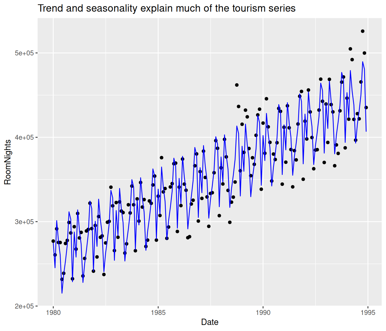
This is a sensible mean model, but the residuals may still be dependent.
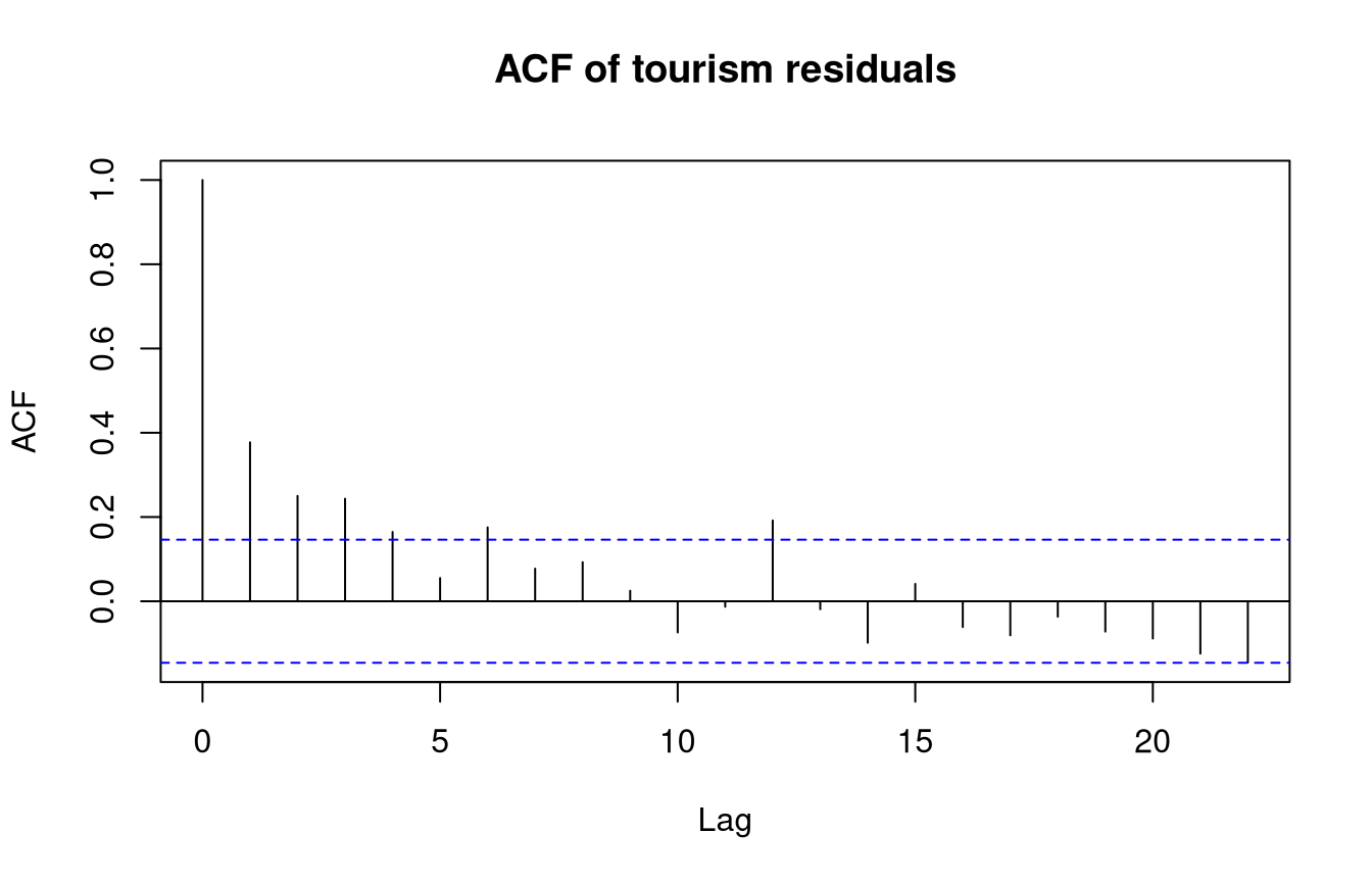
The residual ACF suggests positive autocorrelation, so AR(1) errors are a reasonable first correction.
35.5 Regression Model with AR(1) Errors
For the tourism data we now write \[\begin{aligned} Y_t &= \beta_0 + \beta_1 \mathrm{Time} + \beta_2 z_{t,2} + \cdots + \beta_{12} z_{t,12} + \varepsilon_t, \\ \varepsilon_t &= \phi \varepsilon_{t-1} + \eta_t. \end{aligned}\]
The mean still depends on trend and month. The new ingredient is the correlation structure among the errors.
35.6 Why GLS Works
Suppose \[\begin{aligned} y_t &= \beta_0 + \beta_1 x_t + \varepsilon_t, \\ \varepsilon_t &= \phi \varepsilon_{t-1} + \eta_t. \end{aligned}\]
Subtracting \(\phi\) times the previous equation from the current one gives \[y_t - \phi y_{t-1} = \beta_0(1 - \phi) + \beta_1(x_t - \phi x_{t-1}) + \eta_t.\]
The transformed equation has independent white-noise errors, so it can be handled by least-squares ideas after accounting for the covariance structure. That is the basic idea behind generalized least squares.
35.7 Fitting the AR(1) Model in R
The gls() function from nlme uses the usual model formula plus an explicit correlation structure.
tourism_gls <- gls(RoomNights ~ Time + Month, correlation = corAR1(form = ~Time),
    data = tourism)
anova(tourism_gls)
Denom. DF: 167
numDF F-value p-value
(Intercept) 1 45239.15 <.0001
Time 1 1092.85 <.0001
Month 11 81.94 <.0001Generalized least squares fit by REML
Model: RoomNights ~ Time + Month
Data: tourism
AIC BIC logLik
3727.911 3774.681 -1848.955
Correlation Structure: AR(1)
Formula: ~Time
Parameter estimate(s):
Phi
0.392721
Coefficients:
Value Std.Error t-value p-value
(Intercept) 275492.20 4692.407 58.71021 0.0000
Time 1062.25 31.870 33.33115 0.0000
MonthFeb -31194.09 4205.044 -7.41825 0.0000
MonthMar 23482.73 4959.531 4.73487 0.0000
MonthApr -2170.47 5225.494 -0.41536 0.6784
MonthMay -19419.12 5325.710 -3.64630 0.0004
MonthJun -65827.11 5362.987 -12.27434 0.0000
MonthJul -44522.34 5373.207 -8.28599 0.0000
MonthAug -29768.74 5365.559 -5.54812 0.0000
MonthSep -12039.27 5331.948 -2.25795 0.0252
MonthOct 26393.95 5238.620 5.03834 0.0000
MonthNov 16471.67 4988.022 3.30224 0.0012
MonthDec -58631.94 4272.401 -13.72342 0.0000
Correlation:
(Intr) Time MnthFb MnthMr MnthAp MnthMy MnthJn MnthJl MnthAg MnthSp
Time -0.586
MonthFeb -0.447 0.003
MonthMar -0.525 -0.001 0.589
MonthApr -0.551 -0.005 0.462 0.659
MonthMay -0.558 -0.011 0.416 0.535 0.682
MonthJun -0.559 -0.016 0.398 0.487 0.560 0.690
MonthJul -0.557 -0.022 0.391 0.468 0.512 0.568 0.692
MonthAug -0.552 -0.028 0.387 0.460 0.492 0.520 0.571 0.692
MonthSep -0.545 -0.034 0.383 0.454 0.481 0.498 0.520 0.569 0.690
MonthOct -0.532 -0.039 0.376 0.445 0.470 0.482 0.493 0.513 0.561 0.683
MonthNov -0.502 -0.044 0.358 0.423 0.446 0.456 0.463 0.471 0.491 0.538
MonthDec -0.426 -0.048 0.308 0.364 0.384 0.392 0.396 0.400 0.407 0.425
MnthOc MnthNv
Time
MonthFeb
MonthMar
MonthApr
MonthMay
MonthJun
MonthJul
MonthAug
MonthSep
MonthOct
MonthNov 0.662
MonthDec 0.471 0.597
Standardized residuals:
Min Q1 Med Q3 Max
-2.5656600 -0.6285951 -0.1307054 0.5424996 3.2823396
Residual standard error: 14799.38
Degrees of freedom: 180 total; 167 residualThe argument correlation = corAR1(form = ~ Time) says that adjacent observations in time follow an AR(1) error process.
35.7.1 Comparing OLS and GLS Standard Errors
list(gls = tidy(tourism_gls), lm = tidy(tourism_lm)) |>
    bind_rows(.id = "model") |>
    filter(term == "Time") |>
    select(model, term, estimate, std.error)
# A tibble: 2 × 4
model term estimate std.error
<chr> <chr> <dbl> <dbl>
1 gls Time 1062. 31.9
2 lm Time 1059. 21.2The coefficient estimate for the trend is usually similar, but the standard error can change appreciably once autocorrelation is acknowledged. That is the main reason for fitting the more appropriate model.
35.8 A Short Comparison: Seoul Bike with AR(1) Errors
The same modelling pattern can be used for the daily Seoul bike data once we have already chosen a reasonable mean structure.
seoul_daily <- read_csv("../data/seoul_bike_daily.csv", show_col_types = FALSE) |>
    mutate(S1 = sin(2 * pi * day_index/365), C1 = cos(2 * pi * day_index/365), S2 = sin(4 *
        pi * day_index/365), C2 = cos(4 * pi * day_index/365))

seoul_lm <- lm(rented_bike_count ~ day_index + S1 + C1 + S2 + C2 + mean_temperature +
    total_rainfall + total_solar_radiation, data = seoul_daily)

seoul_gls <- gls(rented_bike_count ~ day_index + S1 + C1 + S2 + C2 + mean_temperature +
    total_rainfall + total_solar_radiation, correlation = corAR1(form = ~day_index),
data = seoul_daily)list(gls = tidy(seoul_gls), lm = tidy(seoul_lm)) |>
bind_rows(.id = "model") |>
filter(term == "day_index") |>
select(model, term, estimate, std.error)# A tibble: 2 × 4
model term estimate std.error
<chr> <chr> <dbl> <dbl>
1 gls day_index 13.9 6.39
2 lm day_index 14.4 5.59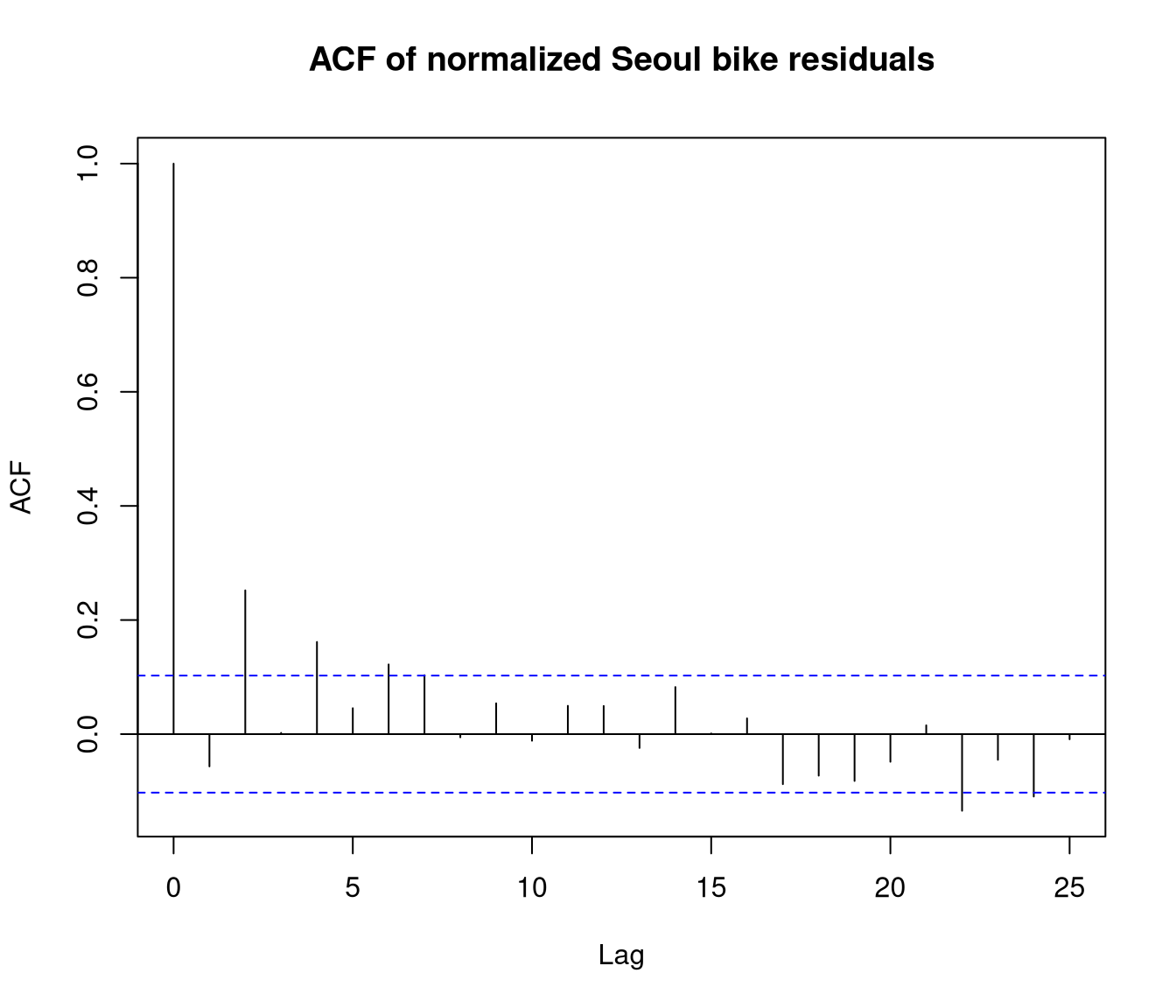
The tourism example shows the method in a classical monthly setting, while the Seoul bike example shows that the same gls(..., correlation = corAR1()) idea carries over directly to a modern daily dataset.