29 Multicollinearity and Ridge Regression
29.1 Idea of Collinearity and Orthogonality
In multiple regression, we often use several explanatory variables at the same time. Sometimes these explanatory variables give us different kinds of information. For example, in a model for electricity bills, the number of people in a house and the area of the house may both be useful predictors. But sometimes explanatory variables overlap strongly. For example, household income and house area may be strongly related. Higher-income households may tend to live in larger houses. If both variables are included in the same model, the regression has to separate two predictors that are partly measuring the same underlying thing.
This problem is called multicollinearity. Multicollinearity occurs when two or more explanatory variables are strongly related to each other. It does not necessarily mean that the model predicts badly. The main problem is that the individual regression coefficients can become hard to interpret.
Consider the model \[Y = \beta_0 + \beta_1 X_1 + \beta_2X_2 + \varepsilon.\] We usually interpret \(\beta_1\) as the rate of change in \(Y\) for a one-unit increase in \(X_1\), holding \(X_2\) constant. That interpretation becomes difficult if \(X_1\) and \(X_2\) usually move together.
If \(X_1\) and \(X_2\) have no linear relationship, they are called orthogonal. Orthogonality makes regression easier to interpret because each predictor is contributing separate information. In practice, explanatory variables are rarely perfectly orthogonal unless the data come from a carefully designed experiment. A little non-orthogonality is usually not a problem.
The problem occurs when predictors are so strongly related that the regression coefficients become unstable. Including or excluding one predictor can substantially change the estimated coefficient of another predictor. Multicollinearity can lead to: large standard errors; coefficients that change a lot when the model is changed slightly; coefficients with unexpected signs; and a model that is useful overall, but with individual coefficients that are hard to interpret. In this lecture, we will look at how multicollinearity affects regression models, how to detect it, and what we might do when it appears.
29.2 A Numerical Example
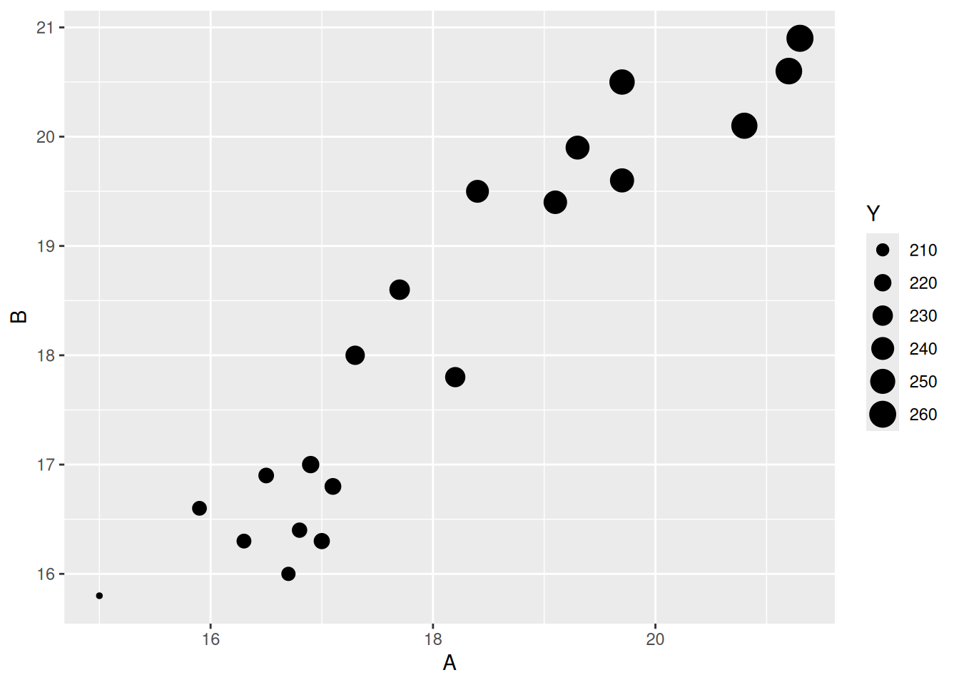
We will consider the effects of multicollinearity using a simple artificial example. Suppose the true model is \[Y = 50 + 5A + 5B + \epsilon.\] Both \(A\) and \(B\) genuinely affect \(Y\). The issue is that \(A\) and \(B\) are highly correlated.
29.2.3 Breaking the correlation
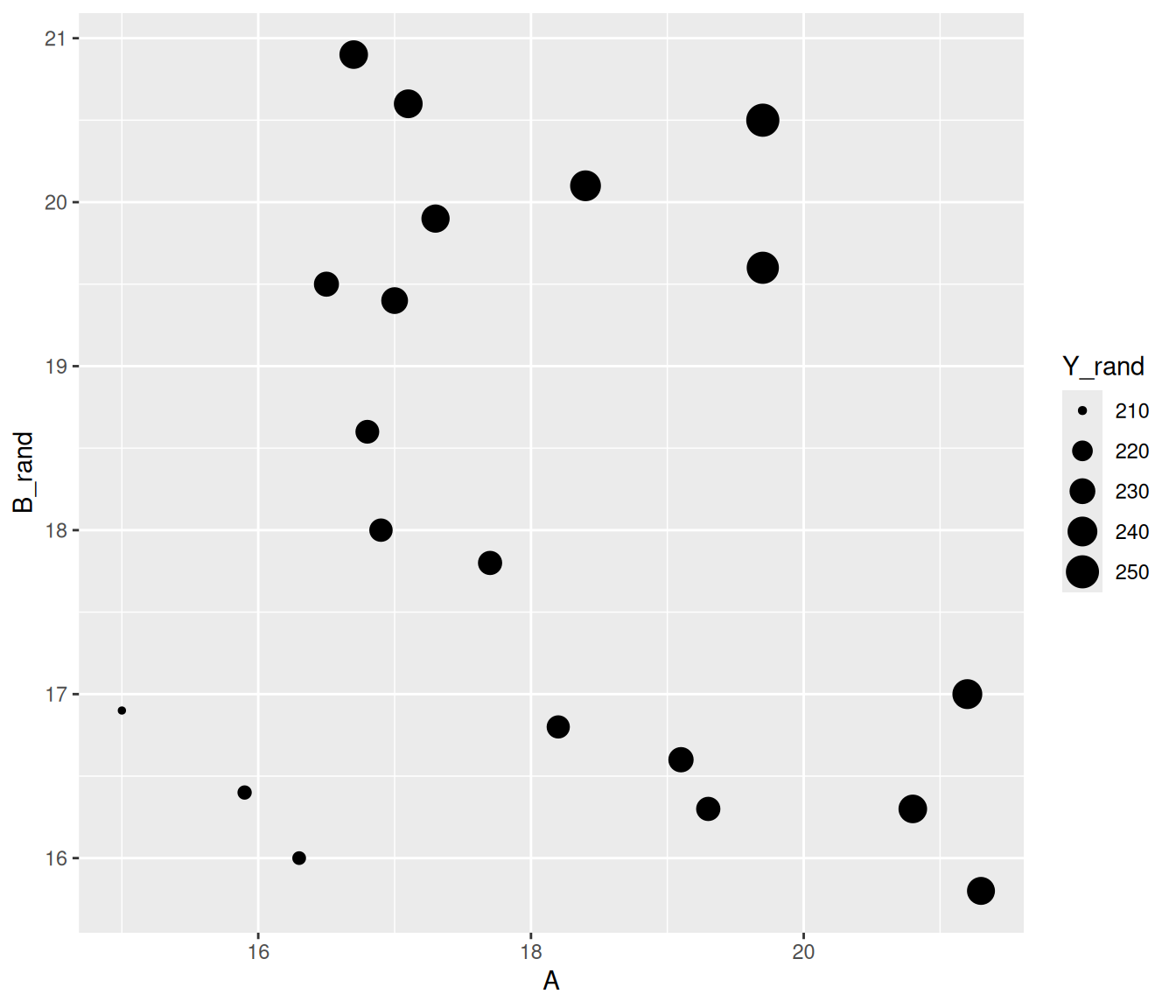
Now suppose we keep the same values of \(A\), \(B\), and \(\epsilon\), but break the correlation between \(A\) and \(B\). One simple way to do this is to randomly reorder the values in column \(B\).
set.seed(42)

sim_rand <- sim_final |>
    mutate(B_rand = sample(B)) |>
    mutate(Y_rand = 50 + 5 * A + 5 * B_rand + epsilon)
Now \(A\) and B_rand contain the same numerical values as before, but the strong relationship between them has been broken.
29.2.5 Orthogonal Data
Consider the model \[Y = \beta_0 + \beta_1 X + \beta_2 Z + \varepsilon\]
Recall that if \(X\) and \(Z\) are uncorrelated, they are called orthogonal. Then
the least squares estimates \(\hat\beta_1\) and \(\hat\beta_2\) are independent of each other
the order of adding the variables does not affect the sums of squares in the ANOVA table.
In other words it doesn’t matter whether we talk about the effect of \(X\) by itself or “\(X\) after \(Z\)”. The effect is the same.
Interpretation of parameters a lot easier.
But it usually only happens in designed experiments with balanced numbers.
In summary, orthogonality of the explanatory variables allows easier interpretation of the results of an experiment and is an important goal in the design of experiments.
29.2.6 Collinear data
Suppose we have three sets of numbers \(X,Z,Y\) such that \[Y = \beta_0 +\beta_1 X + \beta_2 Z +\varepsilon\]
but that, unknown to us, \[Z = \alpha_0 + \alpha_1 X\] at least equal up to some level of rounding error.
Then the regression model could be rewritten in terms of any arbitrary combination of the X and Z figures, as we can always add on \(k\) lots of \(\alpha_0 + \alpha_1 X\) and then take off \(k\) lots of \(Z\) (as they’re the same thing):
\[\begin{aligned}Y &= \beta_0 +\beta_1 X + \beta_2 Z + k(\alpha_0 + \alpha_1 X) - k Z +\varepsilon\\ & = (\beta_0 + k\alpha_0) + (\beta_1 + k\alpha_1)X + (\beta_2 - k)Z + \varepsilon\end{aligned}\]
for any real number \(k\).
There are an infinite number of possible solutions, and if we do get a numerical answer for the regression coefficients, the particular answer may even just depend on rounding, with different amounts of rounding could give very different answers.
29.2.6.1 Not estimable
We describe this situation by saying the regression model is not estimable.
A consequence of such high correlation between the predictor variables is that the regression coefficients may become totally uninterpretable (for example something you know has a positive relationship with the response ends up with a negative coefficient) and the regression coefficients may have very high standard errors.
This is the problem of Multicollinearity.
How do we assess whether it is a real problem in our data?
29.3 Correlations among the predictors
We could look at the correlations between the explanatory variables. Since correlation is a measure of linear relationship, then if two variables are highly correlated then it doesn’t make sense to keep them both in the model.
Example. Consider the data below on household electricity bills with explanatory variables: the income of the household; the number of persons in the house; and the area of the house. Each of these explanatory variables would be expected to be related to the Bill, and yet they are also related to each other, so we may not be able to have them all in the same model.
# A tibble: 34 × 4
    Bill Income Persons  Area
   <dbl>  <dbl>   <dbl> <dbl>
 1   228   3220       2  1160
 2   156   2750       1  1080
 3   648   3620       2  1720
 4   528   3940       1  1840
 5   552   4510       3  2240
 6   636   3990       4  2190
 7   444   2430       1   830
 8   144   3070       1  1150
 9   744   3750       2  1570
10  1104   4790       5  2660
# ℹ 24 more rows
29.3.1 Correlation matrix
We could check all pair-wise correlations with the cor() function:
             Bill    Income   Persons      Area
Bill    1.0000000 0.8368788 0.4941247 0.9050448
Income  0.8368788 1.0000000 0.1426486 0.9612801
Persons 0.4941247 0.1426486 1.0000000 0.3656021
Area    0.9050448 0.9612801 0.3656021 1.0000000
This indicates that the Area of the house is very strongly correlated to the Income of the occupants (\(r= 0.961\)), and so both may say much the same thing about the electricity bill. We may not be able to have both these in the model. By contrast the number of persons in the house is almost unrelated (r = 0.143) to the Income and only weakly related to the Area (r = 0.366) so persons provides more-or-less independent information. A pairs plot can be useful in these circumstances.

29.3.3 Spotting multicollinearity
Call:
lm(formula = Bill ~ Area + Persons + Income, data = electric)

Residuals:
    Min      1Q  Median      3Q     Max
-223.36 -102.88   -8.53   78.61  331.46

Coefficients:
              Estimate Std. Error t value Pr(>|t|)
(Intercept) -358.44157  198.73583  -1.804   0.0813 .
Area           0.28110    0.22611   1.243   0.2234
Persons       55.08763   29.04515   1.897   0.0675 .
Income         0.07514    0.13609   0.552   0.5850
---
Signif. codes:  0 '***' 0.001 '**' 0.01 '*' 0.05 '.' 0.1 ' ' 1

Residual standard error: 135.4 on 30 degrees of freedom
Multiple R-squared:  0.8514,    Adjusted R-squared:  0.8365
F-statistic: 57.28 on 3 and 30 DF,  p-value: 1.585e-12
The regression as a whole is highly significant, yet none of the regression coefficents are significant. This suggests multicollinearity.
29.3.4 Contradictory regression coefficients
Let’s look at the variable we know are highly correlated (i.e. Area and Income) separately as predictors:
By themselves both variables are positively related to Bill and have small Std Errors, as we would expect given the pairs chart.
But let’s see what happens if we put them together:
29.3.4.1 Area and Income together
Call:
lm(formula = Bill ~ Area + Income, data = electric)

Residuals:
   Min     1Q Median     3Q    Max
-221.3 -112.4  -19.8   86.4  297.1

Coefficients:
             Estimate Std. Error t value Pr(>|t|)
(Intercept) -52.23835  120.64872  -0.433    0.668
Area          0.64033    0.12857   4.981 2.27e-05 ***
Income       -0.13498    0.08229  -1.640    0.111
---
Signif. codes:  0 '***' 0.001 '**' 0.01 '*' 0.05 '.' 0.1 ' ' 1

Residual standard error: 141 on 31 degrees of freedom
Multiple R-squared:  0.8336,    Adjusted R-squared:  0.8228
F-statistic: 77.62 on 2 and 31 DF,  p-value: 8.507e-13
When put together, one predictor has changed its sign and the Std Errors are much larger.
This illustrates how multicollinearity can render the regression coefficients quite misleading, as presumably income IS related to higher electricity bills (as folk on higher incomes can afford to have more stuff that consumes energy).
29.3.4.2 Area + Persons model
One solution to multicollinearity is to delete one of the variables. However it can be difficult to decide which one to delete. For example suppose we particularly want to quantify the effect of Persons on the electricity bill after adjusting for one of the others:
elec.lm4 = lm(Bill ~ Area + Persons, data = electric)
elec.lm5 = lm(Bill ~ Income + Persons, data = electric)
summary(elec.lm4)
Call:
lm(formula = Bill ~ Area + Persons, data = electric)

Residuals:
    Min      1Q  Median      3Q     Max
-223.77 -101.97  -13.34   83.17  322.35

Coefficients:
              Estimate Std. Error t value Pr(>|t|)
(Intercept) -255.94923   70.14230  -3.649 0.000959 ***
Area           0.40429    0.03615  11.183 2.08e-12 ***
Persons       42.03394   16.67947   2.520 0.017096 *
---
Signif. codes:  0 '***' 0.001 '**' 0.01 '*' 0.05 '.' 0.1 ' ' 1

Residual standard error: 133.9 on 31 degrees of freedom
Multiple R-squared:  0.8499,    Adjusted R-squared:  0.8402
F-statistic: 87.74 on 2 and 31 DF,  p-value: 1.72e-13
29.3.4.3 Income + Persons model
Call:
lm(formula = Bill ~ Income + Persons, data = electric)

Residuals:
    Min      1Q  Median      3Q     Max
-220.49 -105.87  -22.33   85.43  345.76

Coefficients:
             Estimate Std. Error t value Pr(>|t|)
(Intercept) -575.4106    95.9010  -6.000 1.23e-06 ***
Income         0.2421     0.0222  10.905 3.89e-12 ***
Persons       85.3352    16.0031   5.332 8.28e-06 ***
---
Signif. codes:  0 '***' 0.001 '**' 0.01 '*' 0.05 '.' 0.1 ' ' 1

Residual standard error: 136.6 on 31 degrees of freedom
Multiple R-squared:  0.8437,    Adjusted R-squared:  0.8336
F-statistic: 83.68 on 2 and 31 DF,  p-value: 3.204e-13
Should we estimate that each extra person adds 42 to the electric bill, or 83 to the bill? Of course the interpretation of these regression models differs slightly (in the first model it is the effect of each additional person among families of the same income, while in the second it is the effect of person among families of with homes of the same area). But it still makes one uneasy to see such a big difference.
29.4 Regressing the predictors among themselves
More generally (more than just looking at individual correlations) we could look at whether any of the variables are strongly predicted by a combination of the other regressors. i.e. Whether the \(R^2\) for regressing variable \(X_i\) on the other regressors \(X_1, X_2,..., X_{i-1}, X_{i+1},...,X_{p}\) is large. We call this \(R^2_i\). If it is large then we probably don’t need \(X_i\) (or some other variables) in the model. This is more general than just looking at simple correlations between variables, since the regression model picks up on combinations of variables. A “rule of thumb” is that multicollinearity is a big problem if \(R_i^2 > 0.9\), i.e. the \(i\)th variable is more than 90% explained by the other predictors. We can get \(R_i^2\) by doing the regressions ourselves, but it is easier to consider the concept of variance inflation instead.
29.5 Variance inflation factors, VIFs
A major impact of multicollinearity is found in the variances (and hence standard errors) of the regression coefficients. If \(X_i\) is alone in the model \(Y =\beta_0 +\beta_1 X_i +\varepsilon\), then \(\hat{\mbox{var}}(\hat\beta_1) = \frac{s^2}{(n-1)\mbox{var}(X_i)}\). If \(X_i\) is in a model with other predictors then \(\hat{\mbox{var}}(\hat\beta_i) = s^2 \left(X^T X\right)^{-1}_{ii}\) where the last term is the corresponding diagonal entry of the \((X^T X )^{-1}\) matrix, the variance-covariance matrix.
It turns out that we can rewrite this as: \(\hat{\mbox{var}}(\hat\beta_i) = \frac{s^2}{(n-1)\mbox{var}(X_i)}\cdot \frac{1}{1 - R_i^2}\) where \(R_i^2\) is the multiple \(R^2\) of the regression of \(X_i\) on the other predictors. Thus, when going from a model with just \(X_i\) to a full model, the variance of the coefficent of \(X_i\) inflates by a factor of \(\mbox{VIF}_i = \frac{1}{1 - R_i^2}\). Variable inflation factors that are large (e.g. \(\mbox{VIF}_i > 10\)) indicates multicollinearity problems. On the other hand if the VIF is around 1, then the variable \(X_i\) is pretty much orthogonal to the other variables.
29.5.1 Computing VIFs
To obtain VIFs we need to invoke library(car).
     Area   Persons    Income
44.141264  3.421738 39.035444
Clearly we need to do something to reduce the multicollinearity.
What we do is application-specific! We might choose to remove a variable, or we might choose to do something else (e.g. find a better measure or somehow combine the variables into some average?)
29.6 Example: SAP data
The following example illustrates multicollinearity in a context where it is not immediately visible. Chatterjee and Price discuss a dataset relating Sales S to A (advertising expenditure), A1 (last year’s advertising), P (promotion expenditure), P1 (last year’s promotions expenditure) and SE (sales expenses). The analyst eventually found out that an approximate budgetary constraint
\[ A + A1 + P + P1 = 5 \] was hidden in the data. The constraint was known to the advertising executives who had commissioned the study but it had not been mentioned to the statistical consultant who was given the data to analyze.
# A tibble: 22 × 6
       A     P    SE    A1    P1     S
   <dbl> <dbl> <dbl> <dbl> <dbl> <dbl>
 1  1.99   1    0.3   2.02   0    20.1
 2  1.94   0    0.3   1.99   1    15.1
 3  2.20   0.8  0.35  1.94   0    18.7
 4  2.00   0    0.35  2.20   0.8  16.1
 5  1.69   1.3  0.3   2.00   0    21.3
 6  1.74   0.3  0.32  1.69   1.3  17.8
 7  2.07   1    0.31  1.74   0.3  18.9
 8  1.02   1    0.41  2.07   1    21.3
 9  2.02   0.9  0.45  1.02   1    20.5
10  1.06   1    0.45  2.02   0.9  20.5
# ℹ 12 more rows
29.6.1 SAP full model
We start with a linear model for sales in terms of all other variables:
Call:
lm(formula = S ~ A + P + SE + A1 + P1, data = SAP)

Residuals:
    Min      1Q  Median      3Q     Max
-1.8601 -0.9847  0.1323  0.7017  2.2046

Coefficients:
            Estimate Std. Error t value Pr(>|t|)
(Intercept)  -14.194     18.715  -0.758   0.4592
A              5.361      4.028   1.331   0.2019
P              8.372      3.586   2.334   0.0329 *
SE            22.521      2.142  10.512 1.36e-08 ***
A1             3.855      3.578   1.077   0.2973
P1             4.125      3.895   1.059   0.3053
---
Signif. codes:  0 '***' 0.001 '**' 0.01 '*' 0.05 '.' 0.1 ' ' 1

Residual standard error: 1.32 on 16 degrees of freedom
Multiple R-squared:  0.9169,    Adjusted R-squared:  0.8909
F-statistic:  35.3 on 5 and 16 DF,  p-value: 4.289e-08
29.6.2 SAP VIFs
We see that, apart from Sales Expenses, there is only weak evidence of a relationship between advertising, promotions and sales.
        A         P        SE        A1        P1
36.941513 33.473514  1.075962 25.915651 43.520965
The VIF shows high multicollinearity for all advertising and promotions data.
29.6.3 Dropping variables from SAP
If we drop one of the variables the others change their coefficients unpredictably depending on which variable we drop.
SAP.lm2 = lm(S ~ P + SE + A1 + P1, data = SAP)
SAP.lm3 = lm(S ~ A + P + SE + P1, data = SAP)
SAP.lm2 |>
    tidy()
# A tibble: 5 × 5
term estimate std.error statistic p.value
<chr> <dbl> <dbl> <dbl> <dbl>
1 (Intercept) 10.5 2.46 4.28 0.000510
2 P 3.70 0.757 4.89 0.000138
3 SE 22.8 2.18 10.5 0.00000000804
4 A1 -0.769 0.875 -0.880 0.391
5 P1 -0.969 0.742 -1.31 0.209 # A tibble: 5 × 5
term estimate std.error statistic p.value
<chr> <dbl> <dbl> <dbl> <dbl>
1 (Intercept) 5.76 2.70 2.14 0.0475
2 A 1.15 0.967 1.19 0.252
3 P 4.61 0.830 5.56 0.0000347
4 SE 22.7 2.15 10.6 0.00000000666
5 P1 0.0315 0.862 0.0365 0.971 29.7 What do we do about multicollinearity?
As far as 161.251 is concerned, we have few options.
We can remove one (or more) of the correlated variables from the regression. Our aim is to fix the problem, but sometimes we have a bit of choice which variable to remove, in which case we would like the model to be as interpretable as possible. Sometimes the choice is between a variable with many missing values and one with few, and so we choose the latter if it allows us a bigger effective sample size \(n\).
We could construct another variable which is a combination of the two most highly correlated variables. It might be an ordinary average \((X_1+X_2)/2\), or an average of standardized versions of the \(X_i\)s or some other linear combination. Sometimes subtracting or dividing one variable by another will help. For example the incidence of a particular disease such as obesity may be higher in countries with high GDP and high Population. But GDP depends on the size of the economy, which is correlated with the Population. Dividing gives us per capita GDP which is a better indicator of average wealth and hence may be more related to disease incidence.
We can use penalised regression methods. This links back to the previous lecture.
29.8 Link back to penalised regression
In the previous lecture, we introduced ridge and lasso regression. Both methods add a penalty to the regression fit. Ridge uses an \(L_2\) penalty: \(\lambda \sum_{j=1}^{p}\beta_j^2\). Lasso uses an \(L_1\) penalty: \(\lambda \sum_{j=1}^{p}|\beta_j|\). Both can be useful when predictors overlap, but they behave differently. Ridge keeps the predictors in the model and shrinks their coefficients toward zero. This can help when several predictors carry related information and we do not want the fitted coefficients to become too unstable. Lasso can shrink some coefficients exactly to zero. This can help when we want a smaller selected set of predictors, but it may choose one variable from a group of correlated variables and discard another similar variable. So, when the problem is mainly coefficient instability from overlapping predictors, ridge is often the more natural first example. When the goal is variable selection, lasso is often more natural. Neither method makes correlated observational predictors independent. They are modelling tools, not substitutes for better study design.
29.9 Running example revisited: Seoul bike predictors
In the previous lecture, we used the Seoul bike data to compare stepwise regression, ridge regression, and lasso regression. The conclusion was not that one method clearly won. The training MSE values were very similar. The main difference was how the methods controlled model complexity. Here we return to the same example for a different reason. Instead of asking which method predicts best, we ask: why might the ordinary regression coefficients be unstable? The answer is that some of the predictors overlap in the information they carry. For example, weather variables such as temperature, humidity, dew point, and solar radiation are not independent pieces of information.
                      temperature humidity wind_speed visibility
temperature                  1.00     0.16      -0.04       0.03
humidity                     0.16     1.00      -0.34      -0.54
wind_speed                  -0.04    -0.34       1.00       0.17
visibility                   0.03    -0.54       0.17       1.00
dew_point_temperature        0.91     0.54      -0.18      -0.18
solar_radiation              0.35    -0.46       0.33       0.15
rainfall                     0.05     0.24      -0.02      -0.17
snowfall                    -0.22     0.11       0.00      -0.12
                      dew_point_temperature solar_radiation rainfall snowfall
temperature                            0.91            0.35     0.05    -0.22
humidity                               0.54           -0.46     0.24     0.11
wind_speed                            -0.18            0.33    -0.02     0.00
visibility                            -0.18            0.15    -0.17    -0.12
dew_point_temperature                  1.00            0.09     0.13    -0.15
solar_radiation                        0.09            1.00    -0.07    -0.07
rainfall                               0.13           -0.07     1.00     0.01
snowfall                              -0.15           -0.07     0.01     1.00
The correlation matrix shows that some weather predictors are strongly related. For example, temperature and dew point are strongly correlated. Humidity and visibility are also related. This matters because the regression model tries to estimate the separate effect of each predictor while holding the others constant. That is difficult when the predictors tend to move together.
A pairs plot gives the same idea visually.
library(GGally)

seoul_pairs_data = seoul_hourly |>
    transmute(`Bike count` = rented_bike_count, Temperature = temperature, Humidity = humidity,
        `Dew point` = dew_point_temperature, `Solar radiation` = solar_radiation)

ggpairs(seoul_pairs_data, upper = list(continuous = wrap("cor", size = 4)), lower = list(continuous = wrap("points",
    alpha = 0.12, size = 0.4)), diag = list(continuous = wrap("densityDiag", alpha = 0.35))) +
    theme_bw(base_size = 12) + labs(title = "Seoul bike demand and overlapping weather predictors",
    subtitle = "Strong correlations indicate predictors that may cause unstable regression coefficients")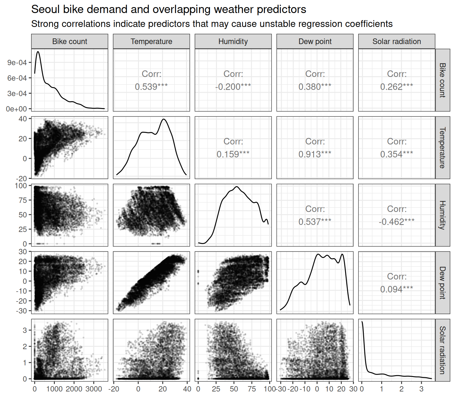
Now fit an ordinary linear model using only the weather predictors.
seoul_weather.lm = lm(rented_bike_count ~ temperature + humidity + dew_point_temperature +
    solar_radiation + rainfall + snowfall, data = seoul_hourly)
summary(seoul_weather.lm)
Call:
lm(formula = rented_bike_count ~ temperature + humidity + dew_point_temperature +
    solar_radiation + rainfall + snowfall, data = seoul_hourly)

Residuals:
     Min       1Q   Median       3Q      Max
-1381.46  -306.28   -46.83   212.51  2439.97

Coefficients:
                      Estimate Std. Error t value Pr(>|t|)
(Intercept)            887.064    100.116   8.860  < 2e-16 ***
temperature             38.101      4.180   9.114  < 2e-16 ***
humidity               -10.294      1.147  -8.976  < 2e-16 ***
dew_point_temperature   -3.061      4.402  -0.696 0.486741
solar_radiation       -100.996      8.322 -12.137  < 2e-16 ***
rainfall               -48.190      4.946  -9.744  < 2e-16 ***
snowfall                42.811     12.865   3.328 0.000879 ***
---
Signif. codes:  0 '***' 0.001 '**' 0.01 '*' 0.05 '.' 0.1 ' ' 1

Residual standard error: 503.1 on 8753 degrees of freedom
Multiple R-squared:  0.392, Adjusted R-squared:  0.3916
F-statistic: 940.7 on 6 and 8753 DF,  p-value: < 2.2e-16
This model may still be useful for prediction, but the individual weather coefficients should be interpreted cautiously. Weather is still relevant, but the predictors overlap so strongly that their separate coefficients are hard to interpret.
We can check this more formally using variance inflation factors.
          temperature              humidity dew_point_temperature
            86.286940             18.872388            114.362629
      solar_radiation              rainfall              snowfall
             1.808663              1.077430              1.092513
Large VIF values tell us that some predictors are strongly explained by the other predictors.
The same Seoul bike model from the previous lecture is not just a model-selection example. It is also a multicollinearity example. In the previous lecture, ridge and lasso were introduced as penalised regression methods. Here, we can now see another reason they are useful. Ridge regression is helpful when we want to keep overlapping predictors in the model but reduce coefficient instability. Lasso regression is helpful when we want to shrink coefficients and possibly remove some predictors. These methods respond to the same problem in different ways. Ridge keeps the overlapping predictors and shrinks their coefficients, whereas lasso may shrink some coefficients all the way to zero. This is why ridge is often discussed in connection with multicollinearity. It is not mainly a variable-selection method. It is a coefficient-stabilisation method.
The important interpretation is: the Seoul bike predictors can give similar prediction accuracy under several methods, but the ordinary regression coefficients may still be unstable because the predictors overlap. Prediction and coefficient interpretation are not the same problem.
29.9.1 Recall from Lecture 28
In the previous lecture we fitted ridge and lasso to the Seoul bike data using glmnet. We used alpha = 0 for ridge regression, and alpha = 1 for lasso regression. We also compared lambda.min and lambda.1se. We do not need to refit those models here. Instead, we focus on why these methods are useful when predictors overlap. Let’s focus on the ridge regression results and compare them to the ordinary regression coefficients.
# A tibble: 7 × 3
  coefficient               OLS   Ridge
  <chr>                   <dbl>   <dbl>
1 (Intercept)            887.   1093.
2 temperature             38.1    23.5
3 humidity               -10.3   -11.8
4 dew_point_temperature   -3.06    9.58
5 solar_radiation       -101.    -61.9
6 rainfall               -48.2   -47.3
7 snowfall                42.8    24.6
Notice how the ridge coefficients are pulled toward zero compared to the OLS estimates. This shrinkage is the mechanism that reduces coefficient instability when predictors overlap.
This is a useful caution. Earlier, in the orthogonal case, ridge had a very simple form: \[\hat\beta^{\text{ridge}}_j = \frac{n}{n+\lambda}\hat\beta^{\text{OLS}}_j.\] That made it look as though every ridge coefficient is just a smaller version of the OLS coefficient. That simple interpretation only holds when the predictors are orthogonal. Here the predictors are not orthogonal. Temperature, humidity, and dew point overlap strongly. In this setting, ridge does not simply shrink each coefficient one at a time. It shrinks the coefficient vector while rebalancing the contributions of correlated predictors. So the ridge coefficient for dew_point_temperature can move away from zero, even though the fitted model is still being penalised. This is why the phrase “ridge shrinks coefficients toward zero” is useful as a first intuition, but not a literal guarantee for every coefficient in a correlated design.
Ridge and lasso both penalise large coefficients. That penalty can reduce the instability caused by multicollinearity. Ridge usually keeps all predictors and shrinks them. Lasso can shrink some predictors exactly to zero. So the same fitted models from the previous lecture can be interpreted in a second way: as tools for controlling model complexity; and as tools for reducing coefficient instability when predictors overlap.
29.10 Lecture Summary
Multicollinearity occurs when explanatory variables overlap in the information they carry. It can produce large standard errors, unstable coefficients, unexpected coefficient signs, and sensitivity to small modelling choices. Correlation matrices and pairs plots can reveal simple pairwise relationships among predictors. Variance inflation factors are a more general diagnostic because they assess how well each predictor can be explained by all the others. One response is to remove or combine correlated predictors. Another response is to use penalised regression. Ridge keeps predictors in the model and shrinks their coefficients toward zero. Lasso shrinks coefficients and can set some exactly to zero. The key point is that multicollinearity is not only a model-selection problem. It is an information problem. If two predictors contain nearly the same information, the data may not be able to tell us cleanly which one is responsible for the association with the response.