28 Stepwise and Penalised Regression
28.1 Automated Variable Selection Procedures
Automated variable selection procedures usually work as follows:
- Choose a starting model, often either the model with no covariates or the model with all covariates included.
- Check whether there is an advantage in adding or removing covariates.
- Repeat this process until there is no clear advantage in changing the model.
28.2 Forward Model Selection
In this technique:
- Fit all one-variable models, and choose the one with the smallest p-value, provided at least one of the simple linear regression models is significant at the chosen significance level.
- Next, fit all two-variable models that include the first chosen X-variable. Choose the variable whose regression coefficient is most significant, provided its p-value is below the chosen cutoff.
- Then fit all three-variable models that include the two variables already chosen, and continue in the same way until there are no more significant variables to add.
- Stop when no further variable meets the entry criterion.
The criterion for “significance” can be chosen by the user. For example, one may decide to only include variables with p-value less than the usual significance level \(\alpha = 0.05\).
28.2.1 When to stop
Sometimes it is useful to allow a higher p-value for entry into the model in forward selection, such as p-value < \(\alpha = 0.25\). This can help us avoid overlooking potentially useful variables. In some settings it is better to cast the net a little wider at first, and then remove weak predictors later.
To decide whether a variable should enter the model, we can look at two equivalent quantities. One option is to check whether the t-value for that variable’s regression coefficient is significant. For example, when df = 60, the t-value will be significant at \(\alpha = 0.05\) if \(|t| > 2\). Because we are comparing two nested models, we can also use the anova() function, for example anova(model_1, model_2), and check whether the F statistic is significant with p-value < 0.05. The two approaches are equivalent when we add just one variable, because \(F = t^2\) where \(F \sim F_{1,df}\).
28.3 Backwards Variable Selection
- Start with a model containing all possible explanatory variables, and possibly interactions as well.
- For each variable in turn, investigate the effect of removing that variable, or interaction if any, from the current model.
- Remove the least informative variable or interaction, unless the term is supplying significant information about the response.
- Go to step 2. Stop only if all variables or interactions in the current model are important.
28.4 Stepwise (direction =“both”)
The phrase stepwise variable selection is usually taken to mean that we start with forward selection, but after each variable is added we check whether any variables already in the model have fallen below the significance criterion \(\alpha\). If so, we remove them. One approach is to use F tests, or equivalently t tests.
28.4.1 Example: Hours of sunshine (backwards)
Use backwards elimination on a full model of Sun from the climate data.
## climate = read.csv("climate.csv", header = TRUE, row.names = 1)
climate.lm1 = lm(Sun ~ ., data = climate)
summary(climate.lm1)
Call:
lm(formula = Sun ~ ., data = climate)

Residuals:
    Min      1Q  Median      3Q     Max
-252.41  -91.95   -2.43   94.71  254.49

Coefficients:
              Estimate Std. Error t value Pr(>|t|)
(Intercept) -5.703e+03  3.809e+03  -1.497   0.1459
Lat         -5.104e+00  2.938e+01  -0.174   0.8634
Long         3.959e+01  1.947e+01   2.033   0.0520 .
MnJanTemp    7.200e+01  4.581e+01   1.572   0.1276
MnJlyTemp   -1.887e+01  3.152e+01  -0.599   0.5544
Rain        -8.373e-02  4.716e-02  -1.775   0.0871 .
Height       2.609e-01  2.833e-01   0.921   0.3652
Sea          2.064e+02  9.785e+01   2.109   0.0443 *
NorthIsland -1.856e+02  1.355e+02  -1.370   0.1820
---
Signif. codes:  0 '***' 0.001 '**' 0.01 '*' 0.05 '.' 0.1 ' ' 1

Residual standard error: 158.7 on 27 degrees of freedom
Multiple R-squared:  0.5843,    Adjusted R-squared:  0.4612
F-statistic: 4.745 on 8 and 27 DF,  p-value: 0.001021
28.4.1.1 Drop Lat
We would drop the variable with the highest p-value, in this case Lat. Only drop one variable at a time. We can use the update() function to save typing.
Call:
lm(formula = Sun ~ Long + MnJanTemp + MnJlyTemp + Rain + Height +
    Sea + NorthIsland, data = climate)

Residuals:
     Min       1Q   Median       3Q      Max
-254.409  -89.690   -3.238   90.960  252.261

Coefficients:
              Estimate Std. Error t value Pr(>|t|)
(Intercept) -6.048e+03  3.193e+03  -1.894   0.0686 .
Long         3.966e+01  1.913e+01   2.073   0.0475 *
MnJanTemp    7.767e+01  3.157e+01   2.460   0.0203 *
MnJlyTemp   -1.671e+01  2.847e+01  -0.587   0.5619
Rain        -8.055e-02  4.271e-02  -1.886   0.0697 .
Height       2.894e-01  2.266e-01   1.277   0.2120
Sea          2.078e+02  9.581e+01   2.169   0.0387 *
NorthIsland -1.777e+02  1.254e+02  -1.417   0.1674
---
Signif. codes:  0 '***' 0.001 '**' 0.01 '*' 0.05 '.' 0.1 ' ' 1

Residual standard error: 155.9 on 28 degrees of freedom
Multiple R-squared:  0.5839,    Adjusted R-squared:  0.4799
F-statistic: 5.613 on 7 and 28 DF,  p-value: 0.000405
28.4.1.2 Drop MnJlyTemp
The highest p-value is now for MnJlyTemp, so we update the model to drop that variable as well. Instead of printing the whole summary, we can use the drop1() function to help decide which variable to drop next.
Single term deletions

Model:
Sun ~ Long + MnJanTemp + Rain + Height + Sea + NorthIsland
            Df Sum of Sq    RSS    AIC F value  Pr(>F)
<none>                   689322 368.96
Long         1     98319 787641 371.76  4.1363 0.05121 .
MnJanTemp    1    140484 829807 373.64  5.9102 0.02147 *
Rain         1    142964 832286 373.74  6.0145 0.02044 *
Height       1     76044 765366 370.73  3.1992 0.08413 .
Sea          1    125566 814888 372.98  5.2826 0.02894 *
NorthIsland  1    107455 796777 372.17  4.5207 0.04212 *
---
Signif. codes:  0 '***' 0.001 '**' 0.01 '*' 0.05 '.' 0.1 ' ' 1
The F test indicates that Height has p-value = 0.08, so we can drop that one as well.
28.4.1.3 Drop Height
Single term deletions

Model:
Sun ~ Long + MnJanTemp + Rain + Sea + NorthIsland
            Df Sum of Sq    RSS    AIC F value  Pr(>F)
<none>                   765366 370.73
Long         1    129226 894592 374.34  5.0653 0.03190 *
MnJanTemp    1     91939 857305 372.81  3.6037 0.06731 .
Rain         1    102527 867893 373.25  4.0188 0.05409 .
Sea          1     54835 820201 371.22  2.1494 0.15303
NorthIsland  1    106633 871999 373.42  4.1797 0.04977 *
---
Signif. codes:  0 '***' 0.001 '**' 0.01 '*' 0.05 '.' 0.1 ' ' 1
Now Sea has p-value = 0.15, so we drop that as well.
28.4.1.4 Drop Sea
Single term deletions

Model:
Sun ~ Long + MnJanTemp + Rain + NorthIsland
            Df Sum of Sq     RSS    AIC F value   Pr(>F)
<none>                    820201 371.22
Long         1    124840  945040 374.32  4.7184 0.037609 *
MnJanTemp    1    209006 1029207 377.39  7.8995 0.008493 **
Rain         1     74019  894219 372.33  2.7976 0.104471
NorthIsland  1    165899  986099 375.85  6.2702 0.017751 *
---
Signif. codes:  0 '***' 0.001 '**' 0.01 '*' 0.05 '.' 0.1 ' ' 1
Finally we drop Rain, which has p-value = 0.10.
28.4.1.5 Drop Rain
Call:
lm(formula = Sun ~ Long + MnJanTemp + NorthIsland, data = climate)

Residuals:
    Min      1Q  Median      3Q     Max
-349.06  -90.02  -15.92   98.84  392.75

Coefficients:
            Estimate Std. Error t value Pr(>|t|)
(Intercept) -7504.65    3290.81  -2.280  0.02938 *
Long           47.33      19.83   2.387  0.02308 *
MnJanTemp      85.06      26.08   3.262  0.00263 **
NorthIsland  -296.09     105.04  -2.819  0.00820 **
---
Signif. codes:  0 '***' 0.001 '**' 0.01 '*' 0.05 '.' 0.1 ' ' 1

Residual standard error: 167.2 on 32 degrees of freedom
Multiple R-squared:  0.4535,    Adjusted R-squared:  0.4023
F-statistic: 8.853 on 3 and 32 DF,  p-value: 0.0002034
We see that annual hours of sunshine are greater in places with high longitude, that is, on the eastern side of New Zealand, and in places with high mean January temperature. The model also suggests, perhaps surprisingly, that hours of sunshine are lower in the North Island. However, NorthIsland and Longitude are correlated, so that apparent effect should be interpreted with care.
28.5 Forward selection
Now try forward selection instead. Do we finish with the same model?
climate.null = lm(Sun ~ 1, data = climate)
add1(climate.null, scope = ~. - Lat + Long + MnJanTemp + MnJlyTemp + Height + Rain +
    Sea + NorthIsland, test = "F")
Single term additions
Model:
Sun ~ 1
Df Sum of Sq RSS AIC F value Pr(>F)
<none> 1636408 388.08
Long 1 344588 1291820 381.57 9.0694 0.004877 **
MnJanTemp 1 506057 1130350 376.76 15.2218 0.000429 ***
MnJlyTemp 1 182734 1453674 385.82 4.2740 0.046380 *
Height 1 90941 1545467 388.02 2.0007 0.166321
Rain 1 316258 1320150 382.35 8.1451 0.007302 **
Sea 1 148252 1488156 386.66 3.3871 0.074450 .
NorthIsland 1 95788 1540620 387.91 2.1140 0.155131
---
Signif. codes: 0 '***' 0.001 '**' 0.01 '*' 0.05 '.' 0.1 ' ' 128.5.0.1 Forward Step 1: Add MnJanTemp
climate.s1 = update(climate.null, . ~ . + MnJanTemp)
add1(climate.s1, scope = ~Lat + Long + MnJanTemp + MnJlyTemp + Height + Rain + Sea +
    NorthIsland, test = "F")
Single term additions
Model:
Sun ~ MnJanTemp
Df Sum of Sq RSS AIC F value Pr(>F)
<none> 1130350 376.76
Lat 1 43712 1086639 377.34 1.3275 0.25753
Long 1 14102 1116248 378.31 0.4169 0.52295
MnJlyTemp 1 22898 1107452 378.03 0.6823 0.41472
Height 1 40 1130310 378.76 0.0012 0.97294
Rain 1 132170 998181 374.29 4.3696 0.04437 *
Sea 1 50284 1080066 377.12 1.5364 0.22390
NorthIsland 1 76944 1053407 376.22 2.4104 0.13007
---
Signif. codes: 0 '***' 0.001 '**' 0.01 '*' 0.05 '.' 0.1 ' ' 128.5.0.2 Forward Step 2: Add Rain
climate.s2 = update(climate.s1, . ~ . + Rain)
add1(climate.s2, scope = ~Lat + Long + MnJanTemp + MnJlyTemp + Height + Rain + Sea +
    NorthIsland, test = "F")
Single term additions
Model:
Sun ~ MnJanTemp + Rain
Df Sum of Sq RSS AIC F value Pr(>F)
<none> 998181 374.29
Lat 1 330 997850 376.27 0.0106 0.91869
Long 1 12081 986099 375.85 0.3921 0.53566
MnJlyTemp 1 16 998165 376.29 0.0005 0.98234
Height 1 1193 996988 376.24 0.0383 0.84612
Sea 1 87195 910985 373.00 3.0629 0.08968 .
NorthIsland 1 53140 945040 374.32 1.7994 0.18923
---
Signif. codes: 0 '***' 0.001 '**' 0.01 '*' 0.05 '.' 0.1 ' ' 1There are no additional variables to add.
28.5.0.3 Forward Selection Final Model
Call:
lm(formula = Sun ~ MnJanTemp + Rain, data = climate)

Residuals:
    Min      1Q  Median      3Q     Max
-353.07  -84.98  -30.65   86.74  383.28

Coefficients:
              Estimate Std. Error t value Pr(>|t|)
(Intercept) 1032.83976  343.96323   3.003  0.00507 **
MnJanTemp     62.40295   19.12695   3.263  0.00257 **
Rain          -0.08159    0.03903  -2.090  0.04437 *
---
Signif. codes:  0 '***' 0.001 '**' 0.01 '*' 0.05 '.' 0.1 ' ' 1

Residual standard error: 173.9 on 33 degrees of freedom
Multiple R-squared:   0.39, Adjusted R-squared:  0.353
F-statistic: 10.55 on 2 and 33 DF,  p-value: 0.0002869
The model chosen by forward selection is different from the one chosen by backwards elimination.
28.5.0.4 Forwards vs Backwards Comparison
Sometimes the two approaches lead to the same model, but in this example they do not. The reason is that two variables can be significant when they appear together in a regression, even if neither is quite strong enough to enter one at a time during forward selection. This is one reason why backwards elimination can sometimes work better.
28.6 Model Selection using AIC
An alternative approach to model selection is to define a numerical measure of model quality and then choose the model that scores best by that measure. The so-called information criteria are examples of such measures. We will look at information criteria in general, the Akaike information criterion (AIC) in particular, and how they can be used for model selection.
28.6.1 Information Criteria
A good regression model should do two things:
- fit the data well;
- remain reasonably simple, with as few predictors as possible.
So we can measure model quality using a quantity of the form \[\mbox{Measure of badness of fit} + k \times \mbox{Number of predictors} + \mbox{constant}\] where k controls the balance between fit and simplicity. Any additive constant is unimportant for model comparison, because it cancels out when we compare different models.
28.6.2 Akaike Information Criterion
Several information criteria in statistics have this general form. One of the most widely used is the Akaike Information Criterion (AIC). For a linear model with unknown error variance, it is defined by \[AIC = n \log (RSS/n) + 2p + \mbox{constant}.\] When comparing models, we prefer the one with the smaller AIC. This is not the only criterion in common use, but it is perhaps the most common.
28.6.3 Back to the Climate data
We have found two different models, climate.lm6 and climate.s2. They have different numbers of variables, and they are not even nested. Even so, we can compare them using the adjusted \(R^2\) or the AIC() function. Both criteria suggest that climate.lm6 is preferred.
[1] 0.4023174[1] 0.3530486[1] 476.4903[1] 478.449728.6.4 AIC in Stepwise Variable Selection
We have seen that sequential variable selection can be carried out using a sequence of F tests. Another option is to compare models using AIC. At each step of the algorithm, we move to the model with the smallest AIC among those formed by adding or dropping a single variable. We stop only when no single addition or deletion reduces AIC further. This procedure is implemented in R by the step() command.
climate.null <- lm(Sun ~ 1, data = climate)
climate.full <- lm(Sun ~ Lat + Long + MnJanTemp + MnJlyTemp + Rain + Height + Sea +
    NorthIsland, data = climate)
scope <- list(lower = formula(climate.null), upper = formula(climate.full))
28.6.4.1 Stepwise Search with step()
Start:  AIC=388.08
Sun ~ 1

              Df Sum of Sq     RSS    AIC
+ MnJanTemp    1    506057 1130350 376.76
+ Long         1    344588 1291820 381.57
+ Rain         1    316258 1320150 382.35
+ Lat          1    220053 1416355 384.88
+ MnJlyTemp    1    182734 1453674 385.82
+ Sea          1    148252 1488156 386.66
+ NorthIsland  1     95788 1540620 387.91
+ Height       1     90941 1545467 388.02
<none>                     1636408 388.08

Step:  AIC=376.76
Sun ~ MnJanTemp

              Df Sum of Sq     RSS    AIC
+ Rain         1    132170  998181 374.29
+ NorthIsland  1     76944 1053407 376.22
<none>                     1130350 376.76
+ Sea          1     50284 1080066 377.12
+ Lat          1     43712 1086639 377.34
+ MnJlyTemp    1     22898 1107452 378.03
+ Long         1     14102 1116248 378.31
+ Height       1        40 1130310 378.76
- MnJanTemp    1    506057 1636408 388.08

Step:  AIC=374.29
Sun ~ MnJanTemp + Rain

              Df Sum of Sq     RSS    AIC
+ Sea          1     87195  910985 373.00
<none>                      998181 374.29
+ NorthIsland  1     53140  945040 374.32
+ Long         1     12081  986099 375.85
+ Height       1      1193  996988 376.24
+ Lat          1       330  997850 376.27
+ MnJlyTemp    1        16  998165 376.29
- Rain         1    132170 1130350 376.76
- MnJanTemp    1    321969 1320150 382.35

Step:  AIC=373
Sun ~ MnJanTemp + Rain + Sea

              Df Sum of Sq     RSS    AIC
+ Height       1     94788  816197 371.04
+ MnJlyTemp    1     52902  858083 372.84
<none>                      910985 373.00
+ Long         1     38986  871999 373.42
- Sea          1     87195  998181 374.29
+ NorthIsland  1     16393  894592 374.34
+ Lat          1      1945  909040 374.92
- Rain         1    169081 1080066 377.12
- MnJanTemp    1    214016 1125001 378.59

Step:  AIC=371.04
Sun ~ MnJanTemp + Rain + Sea + Height

              Df Sum of Sq     RSS    AIC
<none>                      816197 371.04
+ NorthIsland  1     28556  787641 371.76
+ MnJlyTemp    1     22773  793424 372.02
+ Long         1     19420  796777 372.17
+ Lat          1     10788  805409 372.56
- Height       1     94788  910985 373.00
- Sea          1    180791  996988 376.24
- Rain         1    226572 1042769 377.86
- MnJanTemp    1    284136 1100333 379.79
28.6.4.2 Stepwise Model Summary
Call:
lm(formula = Sun ~ MnJanTemp + Rain + Sea + Height, data = climate)

Residuals:
    Min      1Q  Median      3Q     Max
-268.06 -104.31    1.62   90.67  344.42

Coefficients:
            Estimate Std. Error t value Pr(>|t|)
(Intercept) 872.1199   356.7010   2.445  0.02037 *
MnJanTemp    63.9085    19.4541   3.285  0.00253 **
Rain         -0.1123     0.0383  -2.934  0.00625 **
Sea         203.2272    77.5551   2.620  0.01348 *
Height        0.3860     0.2034   1.897  0.06712 .
---
Signif. codes:  0 '***' 0.001 '**' 0.01 '*' 0.05 '.' 0.1 ' ' 1

Residual standard error: 162.3 on 31 degrees of freedom
Multiple R-squared:  0.5012,    Adjusted R-squared:  0.4369
F-statistic: 7.788 on 4 and 31 DF,  p-value: 0.0001822
Notice that AIC is more liberal than the F test here, and it has allowed a non-significant variable into the model.
28.6.5 Backwards elimination via step() and AIC
The syntax below shows how to carry out backwards elimination. This also leaves a non-significant variable in the model, although it gives a higher adjusted R-square.
Start:  AIC=372.48
Sun ~ Lat + Long + MnJanTemp + MnJlyTemp + Rain + Height + Sea +
    NorthIsland

              Df Sum of Sq    RSS    AIC
- Lat          1       760 680941 370.52
- MnJlyTemp    1      9027 689208 370.95
- Height       1     21370 701551 371.59
<none>                     680181 372.48
- NorthIsland  1     47272 727453 372.90
- MnJanTemp    1     62239 742420 373.63
- Rain         1     79398 759579 374.45
- Long         1    104127 784308 375.61
- Sea          1    112082 792263 375.97

Step:  AIC=370.52
Sun ~ Long + MnJanTemp + MnJlyTemp + Rain + Height + Sea + NorthIsland

              Df Sum of Sq    RSS    AIC
- MnJlyTemp    1      8381 689322 368.96
<none>                     680941 370.52
- Height       1     39668 720609 370.56
- NorthIsland  1     48846 729788 371.01
- Rain         1     86487 767428 372.82
- Long         1    104518 785460 373.66
- Sea          1    114410 795351 374.11
- MnJanTemp    1    147165 828106 375.56

Step:  AIC=368.96
Sun ~ Long + MnJanTemp + Rain + Height + Sea + NorthIsland

              Df Sum of Sq    RSS    AIC
<none>                     689322 368.96
- Height       1     76044 765366 370.73
- Long         1     98319 787641 371.76
- NorthIsland  1    107455 796777 372.17
- Sea          1    125566 814888 372.98
- MnJanTemp    1    140484 829807 373.64
- Rain         1    142964 832286 373.74
28.6.5.1 Backwards AIC Model Summary
Call:
lm(formula = Sun ~ Long + MnJanTemp + Rain + Height + Sea + NorthIsland,
    data = climate)

Residuals:
     Min       1Q   Median       3Q      Max
-245.527  -94.201   -9.587   98.988  253.293

Coefficients:
              Estimate Std. Error t value Pr(>|t|)
(Intercept) -5.743e+03  3.114e+03  -1.844   0.0754 .
Long         3.808e+01  1.872e+01   2.034   0.0512 .
MnJanTemp    7.138e+01  2.936e+01   2.431   0.0215 *
Rain        -9.205e-02  3.753e-02  -2.452   0.0204 *
Height       3.527e-01  1.972e-01   1.789   0.0841 .
Sea          1.740e+02  7.571e+01   2.298   0.0289 *
NorthIsland -2.188e+02  1.029e+02  -2.126   0.0421 *
---
Signif. codes:  0 '***' 0.001 '**' 0.01 '*' 0.05 '.' 0.1 ' ' 1

Residual standard error: 154.2 on 29 degrees of freedom
Multiple R-squared:  0.5788,    Adjusted R-squared:  0.4916
F-statistic: 6.641 on 6 and 29 DF,  p-value: 0.0001691
Question: Which of these models is preferred?
28.7 Running Example Bridge: Stepwise Search on Seoul Bike Data
The Seoul bike data give us a more modern example of the same problem. Suppose we want to predict hourly demand from weather and calendar information, but we do not want to hand-build every candidate model.
seoul_subset = seoul_hourly |>
    select(rented_bike_count, hour, season, holiday, functioning_day, temperature,
        humidity, wind_speed, visibility, dew_point_temperature, solar_radiation,
        rainfall, snowfall)

seoul_null = lm(rented_bike_count ~ 1, data = seoul_subset)
seoul_full = lm(rented_bike_count ~ hour + season + holiday + functioning_day + temperature +
    humidity + wind_speed + visibility + dew_point_temperature + solar_radiation +
    rainfall + snowfall, data = seoul_subset)
seoul_scope = list(lower = formula(seoul_null), upper = formula(seoul_full))Single term additions
Model:
rented_bike_count ~ 1
Df Sum of Sq RSS AIC F value Pr(>F)
<none> 3643934363 113342
hour 1 613314401 3030619962 111730 1772.379 < 2.2e-16 ***
season 3 765709006 2878225356 111282 776.468 < 2.2e-16 ***
holiday 1 19067701 3624866661 113298 46.069 1.216e-11 ***
functioning_day 1 151560828 3492373534 112972 380.077 < 2.2e-16 ***
temperature 1 1056904520 2587029843 110343 3577.991 < 2.2e-16 ***
humidity 1 145437128 3498497235 112987 364.082 < 2.2e-16 ***
wind_speed 1 53446519 3590487844 113215 130.368 < 2.2e-16 ***
visibility 1 144710241 3499224121 112989 362.187 < 2.2e-16 ***
dew_point_temperature 1 525597511 3118336852 111980 1476.166 < 2.2e-16 ***
solar_radiation 1 249823064 3394111299 112722 644.631 < 2.2e-16 ***
rainfall 1 55195401 3588738962 113210 134.700 < 2.2e-16 ***
snowfall 1 73273235 3570661128 113166 179.722 < 2.2e-16 ***
---
Signif. codes: 0 '***' 0.001 '**' 0.01 '*' 0.05 '.' 0.1 ' ' 1seoul_step = step(seoul_null, scope = seoul_scope, direction = "both", trace = 0)
formula(seoul_step)rented_bike_count ~ temperature + hour + functioning_day + humidity +
season + rainfall + solar_radiation + holiday + wind_speed +
dew_point_temperature + snowfallThis is exactly the kind of setting where automated search looks tempting:
- there are many plausible predictors,
- some are related to each other,
- and the design can quickly become too large to compare by hand.
The next question is whether we should search by adding and dropping whole terms, or whether we should keep a richer model and shrink the coefficients.
28.8 Penalised Regression: What Actually Happens to the Coefficients?
Stepwise regression makes discrete decisions. A term is either in the model or out of the model. Penalised regression uses a different strategy. We start with a larger model, but discourage the model from using large coefficients. For ordinary least squares, we minimise \[RSS = \sum_{i=1}^{n} (y_i - \hat y_i)^2.\] For penalised regression, we minimise \[RSS + \text{penalty}.\] The penalty is controlled by a tuning parameter \(\lambda\). When \(\lambda = 0\), there is no penalty and we get ordinary least squares. When \(\lambda\) is large, the coefficients are pulled more strongly toward zero. The intercept is usually not penalised. The penalty is applied to the slope coefficients.
28.9 A Clean Case: Orthogonal Predictors
The clearest way to see ridge and lasso is to consider a simple case where the predictors are orthogonal. Orthogonal predictors means that the predictors are uncorrelated with each other in the model matrix. In matrix terms, the columns of \(X\) are perpendicular. Suppose also that the predictors have been centred and scaled so that \[\sum_{i=1}^{n} x_{ij}^{2} = n.\] This is not always true in real data, but it gives a useful clean result.
28.10 Ridge Regression in the Orthogonal Case
Ridge regression minimises \[\sum_{i=1}^{n} \left( y_i - \beta_0 - \sum_{j=1}^{p}\beta_j x_{ij} \right)^2 + \lambda \sum_{j=1}^{p}\beta_j^2.\] The penalty uses squared coefficients. This is called an \(L_2\) penalty. In the orthogonal case, the ridge estimate for each slope coefficient is \[\hat\beta^{\text{ridge}}_j = \frac{n}{n+\lambda} \hat\beta^{\text{OLS}}_j.\] This is the main ridge intuition. Each ordinary least squares coefficient is multiplied by a number between 0 and 1. If \(\lambda = 0\), then \(\frac{n}{n+\lambda} = 1\), so ridge gives the ordinary least squares coefficient. If \(\lambda\) is large, then \(\frac{n}{n+\lambda}\) is closer to 0, so the coefficient is shrunk toward zero. Ridge regression therefore shrinks coefficients, but it usually does not make them exactly zero.
28.11 Lasso Regression in the Orthogonal Case
Lasso regression minimises \[\sum_{i=1}^{n} \left( y_i - \beta_0 - \sum_{j=1}^{p}\beta_j x_{ij} \right)^2 + \lambda \sum_{j=1}^{p}|\beta_j|.\] The penalty uses absolute coefficient values. This is called an \(L_1\) penalty. In the orthogonal case, the lasso estimate is a soft-thresholded version of the ordinary least squares estimate: \[\hat\beta^{\text{lasso}}_j = \text{sign}(\hat\beta^{\text{OLS}}_j) \left( |\hat\beta^{\text{OLS}}_j| - \frac{\lambda}{2n} \right)_+,\] where \((a)_+ = \max(a, 0)\). This formula says: 1. take the ordinary least squares coefficient; 2. reduce its magnitude; 3. if it becomes small enough, set it exactly to zero. That is why lasso can do variable selection. Ridge multiplies coefficients by a shrinkage factor. Lasso subtracts from the absolute size of the coefficient and truncates at zero.
28.12 Why the Geometry Matters
For ridge regression, the constraint has the form \(\beta_1^2 + \beta_2^2 \leq c\). In two dimensions, this is a circle. For lasso regression, the constraint has the form \(|\beta_1| + |\beta_2| \leq c\). In two dimensions, this is a diamond, or a square rotated by 45 degrees. The lasso diamond has corners on the axes. Those corners occur where one coefficient is exactly zero. Because the lasso constraint has corners, the best solution often lands on an axis. When that happens, one coefficient is exactly zero. The ridge constraint is smooth, so the solution is usually shrunk toward zero but not exactly onto an axis. This is the geometric reason that ridge shrinks, while lasso can shrink and select.
library(tidyverse)

theta = seq(0, 2 * pi, length.out = 500)

ridge_boundary = tibble(beta_1 = cos(theta), beta_2 = sin(theta), method = "Ridge: circular L2 constraint")

lasso_boundary = tibble(beta_1 = c(seq(0, 1, length.out = 100), seq(1, 0, length.out = 100),
    seq(0, -1, length.out = 100), seq(-1, 0, length.out = 100)), beta_2 = c(seq(1,
    0, length.out = 100), seq(0, -1, length.out = 100), seq(-1, 0, length.out = 100),
    seq(0, 1, length.out = 100)), method = "Lasso: diamond L1 constraint")

constraint_plot = bind_rows(ridge_boundary, lasso_boundary)

ggplot(constraint_plot, aes(x = beta_1, y = beta_2)) + geom_path(linewidth = 1) +
    facet_wrap(~method) + coord_equal() + labs(x = expression(beta[1]), y = expression(beta[2]),
    title = "Ridge and lasso constraints") + theme_minimal()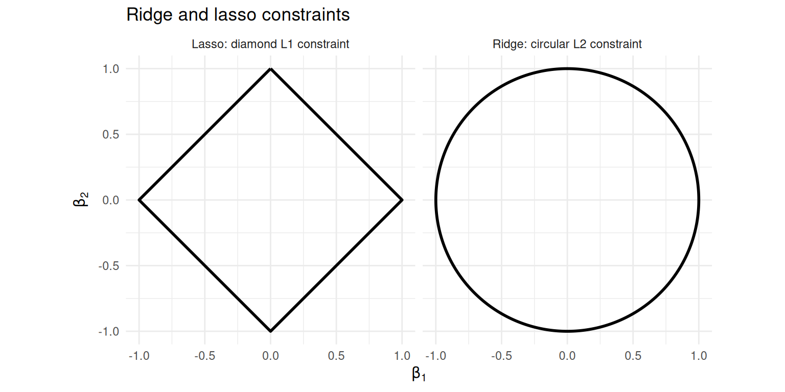
28.13 Why Standardisation Matters
Before ridge or lasso, predictors should usually be standardised. The reason is that the penalty is applied to the coefficient values. Suppose one predictor is measured in metres and another is measured in millimetres. The numerical sizes of their coefficients will be different just because of the measurement scale. Without standardisation, the penalty would not treat the predictors fairly. The glmnet package standardises predictors by default using standardize = TRUE. This is usually what we want for ridge and lasso.
28.14 Using glmnet
The glmnet package fits penalised regression models. It expects the predictors as a numeric matrix and the response as a vector. From this point on, we are treating the problem mainly as prediction, not formal hypothesis testing.
library(glmnet)
library(tidyverse)

X = model.matrix(rented_bike_count ~ hour + season + holiday + functioning_day +
    temperature + humidity + wind_speed + visibility + dew_point_temperature + solar_radiation +
    rainfall + snowfall, data = seoul_subset)[, -1]

y = seoul_subset$rented_bike_count
The model.matrix() function converts the regression formula into the numeric matrix needed by glmnet. It also converts factors into dummy variables. The argument alpha controls the penalty. alpha = 0 gives ridge regression. alpha = 1 gives lasso regression. Values between 0 and 1 give elastic net regression.
28.15 Ridge Regression in glmnet
set.seed(42)

seoul_ridge = cv.glmnet(x = X, y = y, alpha = 0, standardize = TRUE)

plot(seoul_ridge, main = "Ridge regression")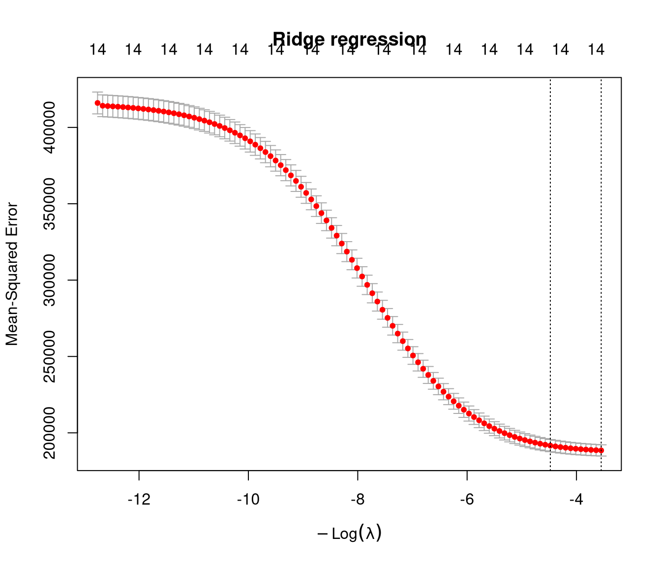
The cross-validation chooses the amount of shrinkage. The value seoul_ridge$lambda.min gives the \(\lambda\) with the smallest cross-validated prediction error. The value seoul_ridge$lambda.1se gives a more strongly penalised model whose error is still within one standard error of the minimum. We can extract the ridge coefficients.
# A tibble: 15 × 3
   coefficient           ridge_lambda_min ridge_lambda_1se
   <chr>                            <dbl>            <dbl>
 1 (Intercept)                  -190.            -213.
 2 hour                           27.1             26.0
 3 seasonSpring                 -103.             -71.5
 4 seasonSummer                  -94.6            -41.4
 5 seasonWinter                 -348.            -320.
 6 holidayNo Holiday             110.             102.
 7 functioning_dayYes            860.             774.
 8 temperature                    16.1             14.1
 9 humidity                       -8.51            -6.98
10 wind_speed                     16.5             15.3
11 visibility                      0.0326           0.0505
12 dew_point_temperature           7.77             6.96
13 solar_radiation               -50.0            -24.5
14 rainfall                      -57.7            -55.0
15 snowfall                       18.7              5.21
Ridge usually keeps all predictors in the model, but reduces the size of the coefficients.
28.16 Lasso Regression in glmnet
set.seed(42)

seoul_lasso = cv.glmnet(x = X, y = y, alpha = 1, standardize = TRUE)

plot(seoul_lasso, main = "Lasso regression")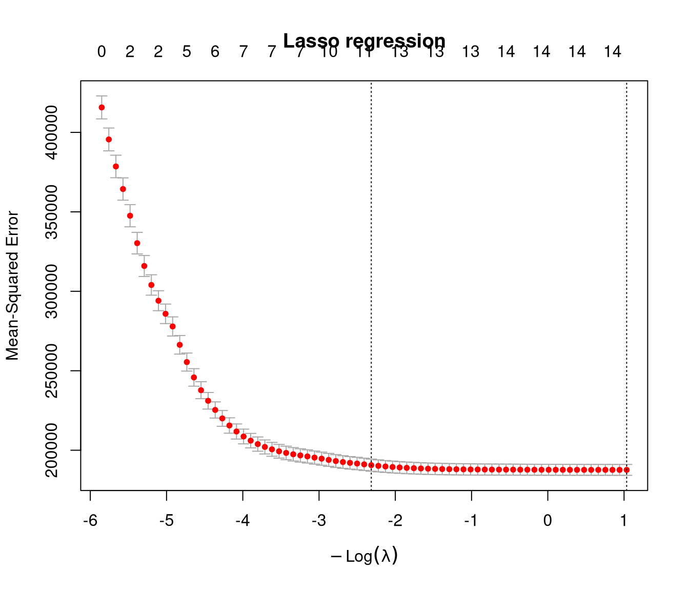
The lasso can set some coefficients exactly to zero.
# A tibble: 15 × 5
   coefficient       lasso_lambda_min lasso_lambda_1se selected_min selected_1se
   <chr>                        <dbl>            <dbl> <lgl>        <lgl>
 1 (Intercept)              -156.            -261.     TRUE         TRUE
 2 hour                       27.5             27.9    TRUE         TRUE
 3 seasonSpring             -133.             -59.5    TRUE         TRUE
 4 seasonSummer             -149.             -22.9    TRUE         TRUE
 5 seasonWinter             -364.            -329.     TRUE         TRUE
 6 holidayNo Holiday         116.              61.7    TRUE         TRUE
 7 functioning_dayY…         928.             818.     TRUE         TRUE
 8 temperature                19.1             21.4    TRUE         TRUE
 9 humidity                   -9.89            -6.57   TRUE         TRUE
10 wind_speed                 18.4              0      TRUE         FALSE
11 visibility                  0.0112           0.0218 TRUE         TRUE
12 dew_point_temper…           7.75             0      TRUE         FALSE
13 solar_radiation           -77.0            -33.0    TRUE         TRUE
14 rainfall                  -58.7            -53.1    TRUE         TRUE
15 snowfall                   30.6              0      TRUE         FALSE
Count the number of selected predictors, excluding the intercept.
Number of non-zero coefficients at lambda.min: 14 Number of non-zero coefficients at lambda.1se: 11 List the selected predictors for each choice.
Selected at lambda.min: [1] "hour" "seasonSpring" "seasonSummer"
[4] "seasonWinter" "holidayNo Holiday" "functioning_dayYes"
[7] "temperature" "humidity" "wind_speed"
[10] "visibility" "dew_point_temperature" "solar_radiation"
[13] "rainfall" "snowfall"
Selected at lambda.1se: [1] "hour" "seasonSpring" "seasonSummer"
[4] "seasonWinter" "holidayNo Holiday" "functioning_dayYes"
[7] "temperature" "humidity" "visibility"
[10] "solar_radiation" "rainfall" The lambda.min model is chosen to minimise cross-validated prediction error. The lambda.1se model is chosen to be more regularised while still having similar prediction error. If lambda.min keeps nearly every variable, that is not a failure of lasso. It means that, for this dataset and this set of predictors, cross-validation found that the less sparse model predicted better.
28.17 Coefficient Path Plot
A coefficient path plot shows how the lasso coefficients change as \(\lambda\) varies.
plot(seoul_lasso$glmnet.fit, xvar = "lambda", label = TRUE)
abline(v = log(seoul_lasso$lambda.min), lty = 2, col = "red")
abline(v = log(seoul_lasso$lambda.1se), lty = 3, col = "blue")
legend("topright", legend = c("lambda.min", "lambda.1se"), lty = c(2, 3), col = c("red",
    "blue"))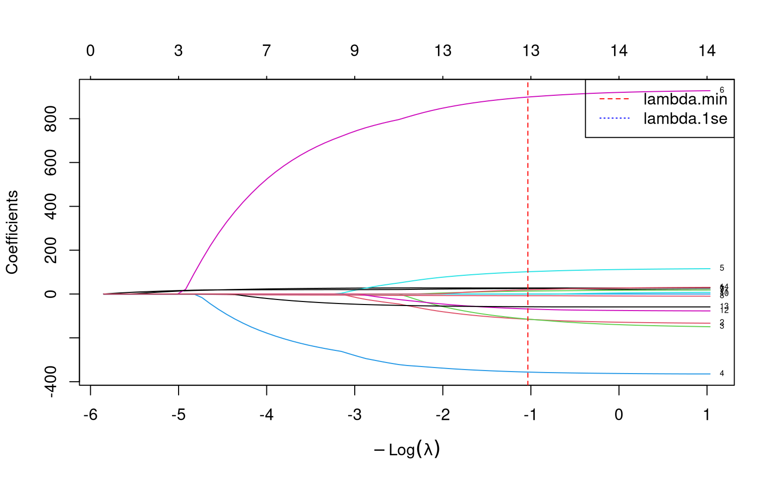
Each line in the plot shows one coefficient. The vertical lines show the two common choices of \(\lambda\). At large \(\lambda\) (left side of the plot), many coefficients are zero. As \(\lambda\) decreases, more coefficients become non-zero.
# A tibble: 2 × 3
  lambda_choice lambda nonzero_predictors
  <chr>          <dbl>              <int>
1 lambda.min     0.356                 14
2 lambda.1se    10.1                   11
28.18 Comparing Stepwise and Lasso
Stepwise regression and lasso are both automated procedures, but they answer slightly different questions. Stepwise regression asks: which terms should be added or removed to improve the model selection criterion? Lasso asks: how much should the coefficients be shrunk, and which coefficients become zero under that amount of shrinkage? For the Seoul bike data, the lasso at lambda.min may keep many or all predictors. That makes it a poor example if our only goal is to show variable selection. But it is a good example for a more realistic point: lasso does not guarantee a tiny model. It produces sparse models only when the cross-validated penalty is strong enough to push some coefficients to zero. In some datasets, many predictors really do contain predictive information. In that case, ridge, lasso, and stepwise selection may give different-looking models because they are controlling complexity in different ways. Let us compare the stepwise formula with the lasso-selected predictors.
Stepwise model terms: [1] "temperature" "hour" "functioning_day"
[4] "humidity" "season" "rainfall"
[7] "solar_radiation" "holiday" "wind_speed"
[10] "dew_point_temperature" "snowfall"
Lasso selected coefficients at lambda.1se: [1] "hour" "seasonSpring" "seasonSummer"
[4] "seasonWinter" "holidayNo Holiday" "functioning_dayYes"
[7] "temperature" "humidity" "visibility"
[10] "solar_radiation" "rainfall"
--- Comparison (mapping lasso dummies back to model terms) ---
In both stepwise and lasso:[1] "temperature" "hour" "functioning_day" "humidity"
[5] "season" "rainfall" "solar_radiation" "holiday"
Only in stepwise (not selected by lasso):[1] "wind_speed" "dew_point_temperature" "snowfall"
Only in lasso (not in stepwise formula):[1] "visibility"Be careful when comparing stepwise and lasso here. Stepwise works with model terms. For example, season is one model term. glmnet works with columns of the model matrix. A factor such as season becomes several dummy-variable columns. So the lasso count is a count of selected columns, not necessarily a count of selected scientific variables.
28.19 MSE Comparison Across Methods
We can compare the fitted performance of each method by computing the mean squared error on the training data.
# A tibble: 5 × 6
  Method                 MSE  RMSE `Non-zero predictors` delta_MSE delta_RMSE
  <chr>                <dbl> <dbl>                 <dbl>     <dbl>      <dbl>
1 Stepwise (AIC)     187028.  432.                    13      2.71    0.00313
2 Ridge (lambda.min) 188027.  434.                    14   1001.      1.16
3 Ridge (lambda.1se) 191245.  437.                    14   4220.      4.85
4 Lasso (lambda.min) 187026.  432.                    14      0       0
5 Lasso (lambda.1se) 190183.  436.                    11   3157.      3.64
The first thing to notice is that the training MSE values are very similar. The RMSE column puts the errors in the original units: bikes per hour. All five models have an RMSE around 432 bikes per hour. The differences between them are only a few bikes per hour. The lowest training RMSE is for lasso at lambda.min (432.3 bikes/hour), but it is almost identical to the stepwise AIC model (432.4 bikes/hour). The difference of 0.1 bikes per hour is practically meaningless. The ridge models have slightly higher RMSE (433.6 and 437.3 bikes/hour). This is expected, because ridge deliberately shrinks coefficients. It is not trying to minimise the training RSS as aggressively as ordinary least squares. Ridge accepts a small loss in training fit in exchange for potentially more stable predictions on new data. The lasso at lambda.min keeps all 14 model-matrix predictors. In this example, lasso at lambda.min is therefore not giving a sparse model. It is mainly acting as a shrinkage method. The lasso at lambda.1se is more interesting for variable selection. It keeps 11 predictors and has an RMSE of 436.1 bikes/hour, only about 4 bikes/hour higher than the best model. This illustrates the usual trade-off: a simpler model may have slightly worse fitted performance, but may be easier to interpret and may generalise better. The number of non-zero predictors should be interpreted carefully. Ridge regression usually does not set coefficients exactly to zero, so the ridge models keep all predictors. Also, glmnet works with columns of the model matrix, whereas stepwise regression works with model terms. A categorical variable can therefore count as one term in stepwise regression but several dummy-variable columns in glmnet. The main conclusion is not that one method clearly wins. Instead, the table shows that several different modelling strategies can give very similar fitted accuracy, while producing different levels of shrinkage and different apparent model complexity. In practice, we would prefer to compare these methods using a held-out test set or cross-validated prediction error, rather than training MSE. Training MSE is useful for illustration, but it is not a fair estimate of future predictive performance. The Seoul bike example shows that penalised regression does not automatically give a dramatically better or much smaller model. Its value is that it gives a principled way to trade off fit, shrinkage, stability, and sparsity.
28.20 Key Takeaway
Penalised regression gives us another way to control model complexity. Instead of searching through many candidate models, we fit a richer model and penalise large coefficients. Ridge regression uses an \(L_2\) penalty and shrinks coefficients toward zero. Lasso regression uses an \(L_1\) penalty and can shrink coefficients exactly to zero. In glmnet, ridge is fitted with alpha = 0, lasso with alpha = 1, and the amount of shrinkage is controlled by \(\lambda\), usually chosen by cross-validation.