34 Diagnosing Autocorrelated Errors
34.2 What Is Autocorrelation?
In ordinary regression, uncorrelated errors mean that once the model has explained the systematic structure, a positive residual on one row tells us nothing about the sign of the next residual.
If nearby residuals tend to be similar, the errors are positively autocorrelated. This gives the familiar long, slow wandering pattern. If nearby residuals tend to alternate above and below zero, the errors are negatively autocorrelated.
Autocorrelation can appear because:
- an important time-related variable has been omitted,
- the response really does have carry-over behaviour,
- or both.
Why does this matter? Least-squares coefficients can still be unbiased, but the reported standard errors are often too small. That makes confidence intervals too narrow and tests too optimistic.
34.3 A Classical Example: Consumer Expenditure and Money Stock
This example studies consumer expenditure (ConsExp) and the stock of money (MoneyStk) in billions of US dollars.
| Year | Quarter | ConsExp | MoneyStk | Year.Q |
|---|---|---|---|---|
| 1952 | 1 | 214.6 | 159.3 | 1952.00 |
| 1952 | 2 | 217.7 | 161.2 | 1952.25 |
| 1952 | 3 | 219.6 | 162.8 | 1952.50 |
| 1952 | 4 | 227.2 | 164.6 | 1952.75 |
| 1953 | 1 | 230.9 | 165.9 | 1953.00 |
| 1953 | 2 | 233.3 | 167.9 | 1953.25 |

34.3.1 Fit the Regression Model
Call:
lm(formula = ConsExp ~ MoneyStk, data = MoneyStock)

Residuals:
   Min     1Q Median     3Q    Max
-7.176 -3.396  1.396  2.928  6.361

Coefficients:
             Estimate Std. Error t value Pr(>|t|)
(Intercept) -154.7192    19.8500  -7.794 3.54e-07 ***
MoneyStk       2.3004     0.1146  20.080 8.99e-14 ***
---
Signif. codes:  0 '***' 0.001 '**' 0.01 '*' 0.05 '.' 0.1 ' ' 1

Residual standard error: 3.983 on 18 degrees of freedom
Multiple R-squared:  0.9573,    Adjusted R-squared:  0.9549
F-statistic: 403.2 on 1 and 18 DF,  p-value: 8.988e-14
At first glance this looks like a useful regression. The fitted line is strong, and the standard output suggests a precise estimate of the slope. But that depends on the residual assumptions being correct.
34.3.2 Residual Plot Over Time
plot(residuals(MoneyStock_lm1), type = "b", ylab = "Residuals", xlab = "Quarter")
abline(h = 0, lty = 2)
The residuals show the long, slow wandering pattern typical of positive autocorrelation. Extended sequences of positive or negative residuals should not be common if the errors are independent.
34.4 Diagnostic Tools
34.4.1 Runs Test
The runs test looks only at the signs of the residuals and asks whether the sequence of plus and minus signs looks random.
    Runs Test for Randomness

data:  residuals(MoneyStock_lm1)
runs = 5, m = 10, n = 10, p-value = 0.008985
alternative hypothesis: true number of runs is not equal the expected number
sample estimates:
median(x)
 1.395704
A small p-value suggests the residuals are not appearing in random order.
34.4.2 Durbin-Watson Test
The Durbin-Watson test is a classical test for first-order autocorrelation in regression residuals.
    Durbin-Watson test

data:  MoneyStock_lm1
DW = 0.32821, p-value = 2.303e-08
alternative hypothesis: true autocorrelation is greater than 0
Here the one-sided alternative reflects the suspicion of positive autocorrelation.
34.4.3 ACF Plot
The autocorrelation function (ACF) shows the correlation between residuals separated by different time lags.
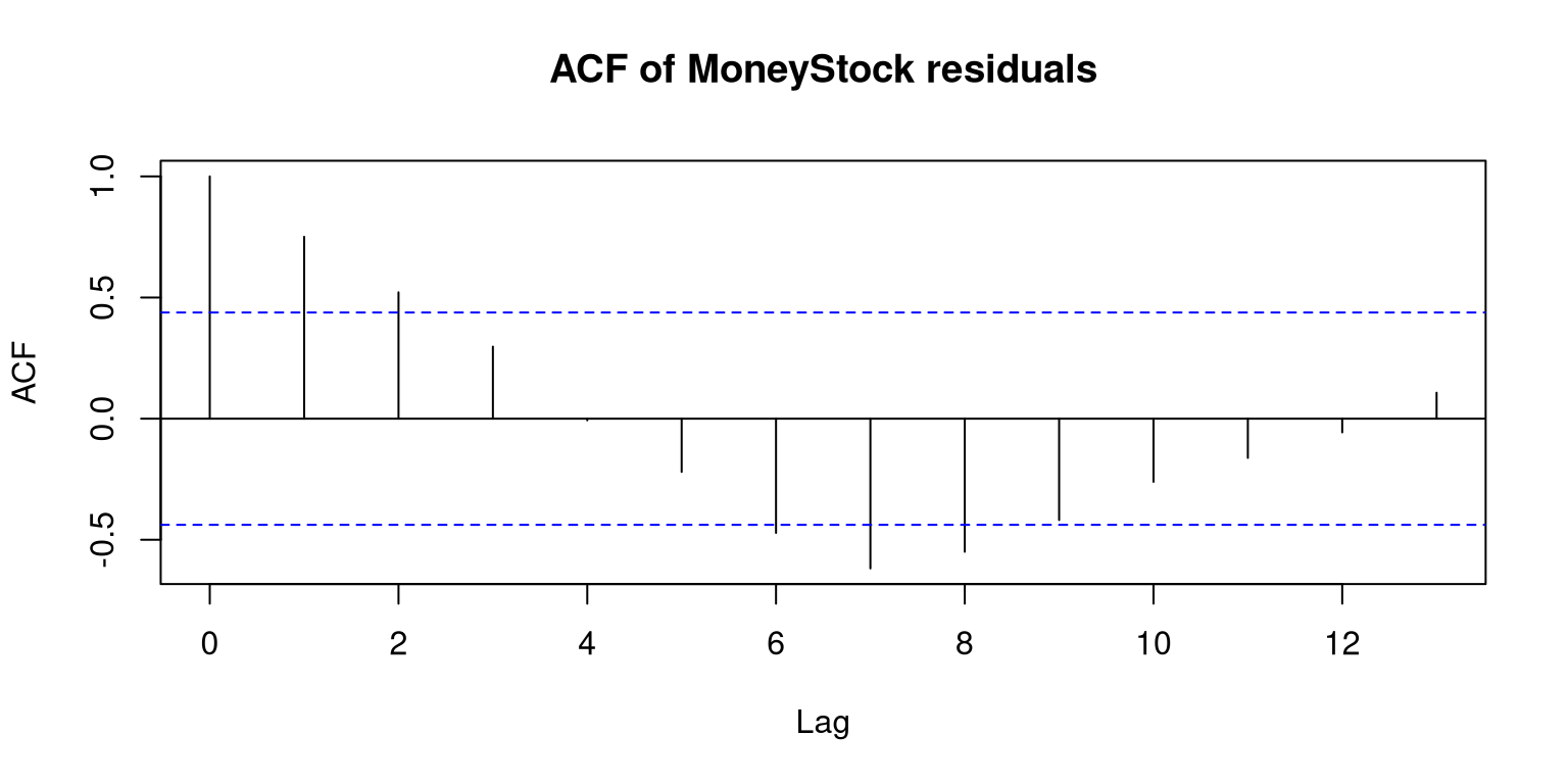
When the lag-1 autocorrelation is substantial, later lags often look large as well because nearby residuals carry information forward through time. A slow decay in the ACF is strong visual evidence that independence is failing.
34.4.4 Ljung-Box Test
The Ljung-Box test checks several autocorrelations at once rather than focusing only on lag 1.
    Box-Ljung test

data:  residuals(MoneyStock_lm1)
X-squared = 64.397, df = 10, p-value = 5.286e-10
If this test rejects, the residual series still contains dependence structure that the fitted regression has not explained.
34.5 A Modern Comparison: Seoul Bike Residuals
The same diagnostic logic applies to the daily bike model from the previous lecture.
seoul_daily <- read_csv("../data/seoul_bike_daily.csv", show_col_types = FALSE) |>
    mutate(S1 = sin(2 * pi * day_index/365), C1 = cos(2 * pi * day_index/365), S2 = sin(4 *
        pi * day_index/365), C2 = cos(4 * pi * day_index/365))

seoul_mean <- lm(rented_bike_count ~ day_index + S1 + C1 + S2 + C2 + mean_temperature +
total_rainfall + total_solar_radiation, data = seoul_daily)plot(residuals(seoul_mean) ~ seoul_daily$day_index, type = "b", ylab = "Residuals",
xlab = "Day index")
abline(h = 0, lty = 2)
    Runs Test for Randomness

data:  residuals(seoul_mean)
z = -5.5558, runs = 130, m = 183, n = 182, p-value = 2.763e-08
alternative hypothesis: true number of runs is not equal the expected number
sample estimates:
median(x)
 474.7272
    Durbin-Watson test

data:  seoul_mean
DW = 1.7794, p-value = 0.007159
alternative hypothesis: true autocorrelation is greater than 0
    Box-Ljung test

data:  residuals(seoul_mean)
X-squared = 64.679, df = 14, p-value = 1.745e-08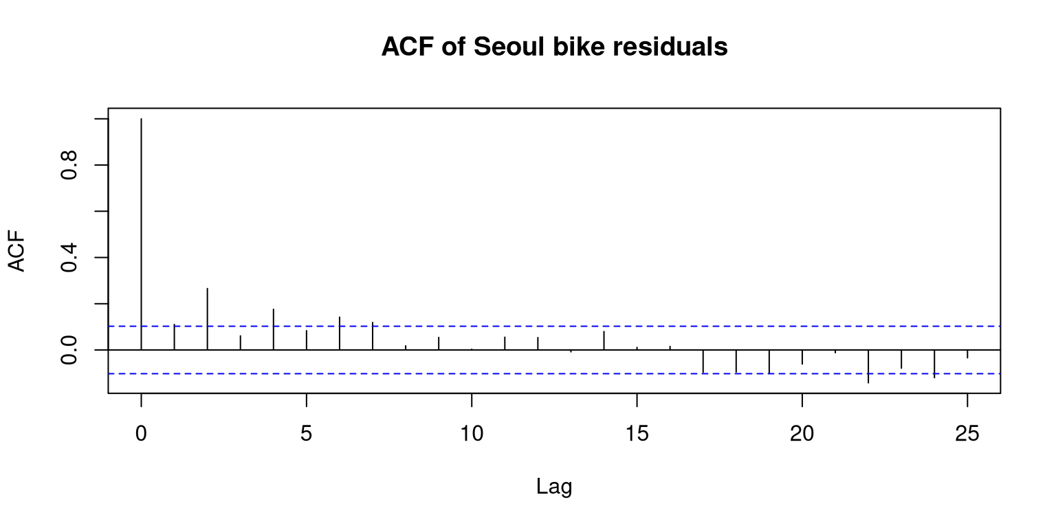
Although the bike model has a much richer mean structure than the MoneyStock regression, the same pattern can still remain: long runs in the residual plot, slow decay in the ACF, and small p-values from formal tests.
34.6 Diagnostic Summary
When several of the following point in the same direction,
- the residual plot shows long runs,
- the runs test rejects randomness,
- the Durbin-Watson test rejects independence,
- the ACF decays slowly,
- and the Ljung-Box test rejects white noise,
we should stop treating the errors as independent.