33 Regression Models for Trend and Seasonality
33.1 Regression Models for Trend and Seasonality
In the previous lecture, a simple seasonal indicator was enough for the ski-sales data. In other situations, the pattern across the year is smoother and more complicated. We want a model that is more flexible than a single winter indicator, but more parsimonious than fitting a separate effect for every month.
By the end of this lecture, students should be able to:
- Use factor indicators to represent seasonality.
- Build sine and cosine predictors for periodic behaviour.
- Explain why sine-plus-cosine allows an unknown phase shift.
- Recognise Fourier terms as a systematic version of the same idea.
33.2 Electricity Bills: Month Effects and Seasonal Shape
We consider monthly electricity bills for a household from May 1994 to May 1998. During some months there were paying guests staying in part of the house, so the householder wanted to estimate the extra business-related electricity cost.
After allowing for the number of days in the bill, whether the bill was estimated, the guest weeks, and a time trend, we then examine what seasonal structure remains.
| Bill | Days | Estimate | Guestwks | Month | Monthlab | Time | Year |
|---|---|---|---|---|---|---|---|
| 70.18 | 29 | 0 | 0 | 5 | M | 5 | 94 |
| 79.05 | 30 | 1 | 0 | 6 | J | 6 | 94 |
| 78.60 | 27 | 0 | 0 | 7 | J | 7 | 94 |
| 81.45 | 29 | 1 | 0 | 8 | A | 8 | 94 |
| 174.25 | 28 | 0 | 4 | 9 | S | 9 | 94 |
| 115.20 | 28 | 1 | 0 | 10 | O | 10 | 94 |
33.2.1 Residual Seasonality After Basic Adjustment
Electricity_lm1 <- lm(Bill ~ Days + Estimate + Guestwks + Time, data = Electricity)
resids <- resid(Electricity_lm1)

plot(resids ~ Time, data = Electricity, ylab = "Residuals")
lines(resids ~ Time, data = Electricity, col = 4)
abline(h = 0, lty = 2)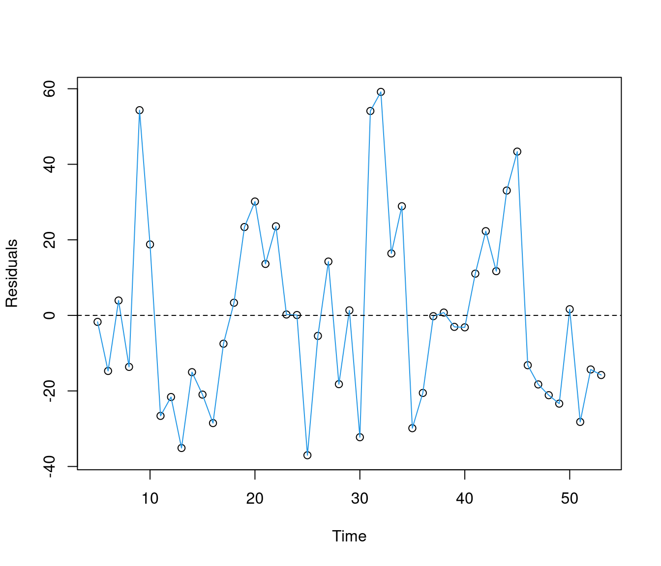
The plot suggests that some months tend to lie above zero and others below zero, so there is still seasonal structure after adjusting for the non-weather-related variables.
33.2.2 A Separate Effect for Each Month
Call:
lm(formula = resids ~ factor(Month), data = Electricity)

Residuals:
    Min      1Q  Median      3Q     Max
-40.822 -11.236   0.350   9.064  31.986

Coefficients:
                Estimate Std. Error t value Pr(>|t|)
(Intercept)      -23.929      8.953  -2.673 0.011125 *
factor(Month)2    19.410     12.661   1.533 0.133785
factor(Month)3    14.437     12.661   1.140 0.261517
factor(Month)4     7.877     12.661   0.622 0.537669
factor(Month)5    21.401     12.012   1.782 0.083015 .
factor(Month)6    18.597     12.661   1.469 0.150341
factor(Month)7    47.215     12.661   3.729 0.000642 ***
factor(Month)8    51.110     12.661   4.037 0.000262 ***
factor(Month)9    55.853     12.661   4.411 8.54e-05 ***
factor(Month)10   38.446     12.661   3.036 0.004368 **
factor(Month)11    5.300     12.661   0.419 0.677957
factor(Month)12    8.133     12.661   0.642 0.524586
---
Signif. codes:  0 '***' 0.001 '**' 0.01 '*' 0.05 '.' 0.1 ' ' 1

Residual standard error: 17.91 on 37 degrees of freedom
Multiple R-squared:  0.5794,    Adjusted R-squared:  0.4543
F-statistic: 4.633 on 11 and 37 DF,  p-value: 0.0002005
This shows that the average residual differs by month. That is useful diagnostically, but using eleven indicator variables for a short series is not very parsimonious.
33.3 Sinusoidal Terms
A smoother alternative is to represent seasonality by sine and cosine waves. Suppose we try \[\sin\left(\frac{2\pi (t - c)}{12}\right)\] for monthly data, where the shift constant \(c\) says where the cycle starts.
An initial guess is to place the zero point near April, because that is close to autumn and might correspond to an “average” month for electricity use.
So we create \[\mathrm{SinTime} = \sin\left(\frac{2\pi (Time - 4)}{12}\right), \qquad \mathrm{CosTime} = \cos\left(\frac{2\pi (Time - 4)}{12}\right).\]
The cosine term matters because we may not know the best phase shift in advance. If the true seasonal pattern is \[A\sin(x + \phi),\] then trigonometry gives \[A\sin(x + \phi) = A\sin(x)\cos(\phi) + A\cos(x)\sin(\phi) = A_1 \sin(x) + A_2 \cos(x).\]
So a regression on both sine and cosine can estimate the amplitude and the phase shift automatically.
33.3.1 First Guess: Shift by Four Months
Electricity <- Electricity |>
    mutate(SinTime = sin((Time - 4) * 2 * pi/12), CosTime = cos((Time - 4) * 2 *
        pi/12))

Electricity_lm3 <- lm(resids ~ SinTime + CosTime, data = Electricity)
summary(Electricity_lm3)
Call:
lm(formula = resids ~ SinTime + CosTime, data = Electricity)

Residuals:
    Min      1Q  Median      3Q     Max
-43.135 -10.729  -2.141  11.561  37.675

Coefficients:
              Estimate Std. Error t value Pr(>|t|)
(Intercept)  -0.003126   2.756424  -0.001  0.99910
SinTime      18.692200   3.917615   4.771 1.89e-05 ***
CosTime     -10.615094   3.878633  -2.737  0.00879 **
---
Signif. codes:  0 '***' 0.001 '**' 0.01 '*' 0.05 '.' 0.1 ' ' 1

Residual standard error: 19.29 on 46 degrees of freedom
Multiple R-squared:  0.3932,    Adjusted R-squared:  0.3669
F-statistic: 14.91 on 2 and 46 DF, p-value: 1.022e-05plot(resids ~ Time, data = Electricity, ylab = "Residuals")
lines(resids ~ Time, data = Electricity, col = 4)
lines(Electricity_lm3$fitted.values ~ Time, data = Electricity, col = 2, lwd = 2,
lty = 2)
abline(h = 0, lty = 2)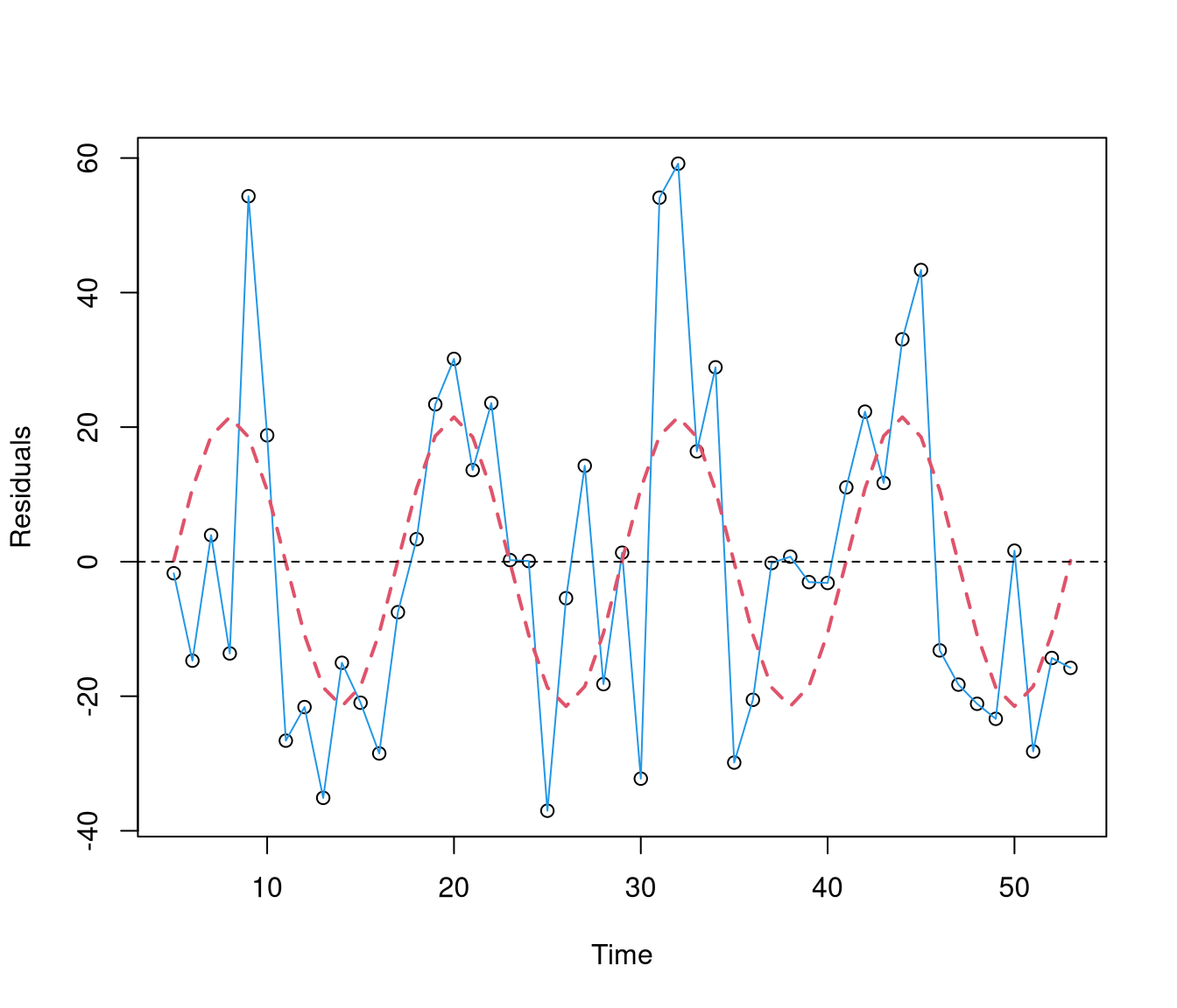
The coefficient of CosTime is clearly not zero, which tells us our guessed phase shift is not quite right.
33.3.2 Second Guess: Shift by Five Months
The fitted curve crosses zero closer to Time = 5, so we try that shift instead.
Electricity <- Electricity |>
    mutate(SinTime = sin((Time - 5) * 2 * pi/12), CosTime = cos((Time - 5) * 2 *
        pi/12))

Electricity_lm4 <- lm(resids ~ SinTime + CosTime, data = Electricity)
summary(Electricity_lm4)
Call:
lm(formula = resids ~ SinTime + CosTime, data = Electricity)

Residuals:
    Min      1Q  Median      3Q     Max
-43.135 -10.729  -2.141  11.561  37.675

Coefficients:
             Estimate Std. Error t value Pr(>|t|)
(Intercept) -0.003126   2.756424  -0.001    0.999
SinTime     21.495467   3.936961   5.460 1.85e-06 ***
CosTime      0.153159   3.858994   0.040    0.969
---
Signif. codes:  0 '***' 0.001 '**' 0.01 '*' 0.05 '.' 0.1 ' ' 1

Residual standard error: 19.29 on 46 degrees of freedom
Multiple R-squared:  0.3932,    Adjusted R-squared:  0.3669
F-statistic: 14.91 on 2 and 46 DF,  p-value: 1.022e-05
Now the cosine term is no longer doing much work, which suggests the revised phase shift is much more sensible.
33.3.3 A Sharper Seasonal Shape: Add Second Harmonics
The fitted curve still looks a little too smooth. In particular, the rise toward winter is steeper than a simple sine wave suggests, so we add terms with twice the frequency: \[\sin\left(\frac{4\pi (Time - 5)}{12}\right), \qquad \cos\left(\frac{4\pi (Time - 5)}{12}\right).\]
Electricity <- Electricity |>
    mutate(Sin2Time = sin((Time - 5) * 4 * pi/12), Cos2Time = cos((Time - 5) * 4 *
        pi/12))

Electricity_lm5 <- lm(resids ~ SinTime + CosTime + Sin2Time + Cos2Time, data = Electricity)
summary(Electricity_lm5)
Call:
lm(formula = resids ~ SinTime + CosTime + Sin2Time + Cos2Time,
    data = Electricity)

Residuals:
    Min      1Q  Median      3Q     Max
-46.043 -13.531   0.651  11.336  34.987

Coefficients:
            Estimate Std. Error t value Pr(>|t|)
(Intercept)   0.2067     2.4900   0.083  0.93423
SinTime      21.4955     3.5550   6.046 2.88e-07 ***
CosTime       0.5727     3.4873   0.164  0.87030
Sin2Time     -6.1586     3.5550  -1.732  0.09022 .
Cos2Time    -10.6995     3.4873  -3.068  0.00368 **
---
Signif. codes:  0 '***' 0.001 '**' 0.01 '*' 0.05 '.' 0.1 ' ' 1

Residual standard error: 17.42 on 44 degrees of freedom
Multiple R-squared:  0.5268,    Adjusted R-squared:  0.4837
F-statistic: 12.24 on 4 and 44 DF, p-value: 8.949e-07Analysis of Variance Table
Model 1: resids ~ SinTime + CosTime
Model 2: resids ~ SinTime + CosTime + Sin2Time + Cos2Time
Res.Df RSS Df Sum of Sq F Pr(>F)
1 46 17112
2 44 13346 2 3765.5 6.2072 0.004221 **
---
Signif. codes: 0 '***' 0.001 '**' 0.01 '*' 0.05 '.' 0.1 ' ' 1plot(resids ~ Time, data = Electricity, ylab = "Residuals")
lines(resids ~ Time, data = Electricity, col = 4)
lines(Electricity_lm5$fitted.values ~ Time, data = Electricity, col = 2, lwd = 2,
lty = 2)
abline(h = 0, lty = 2)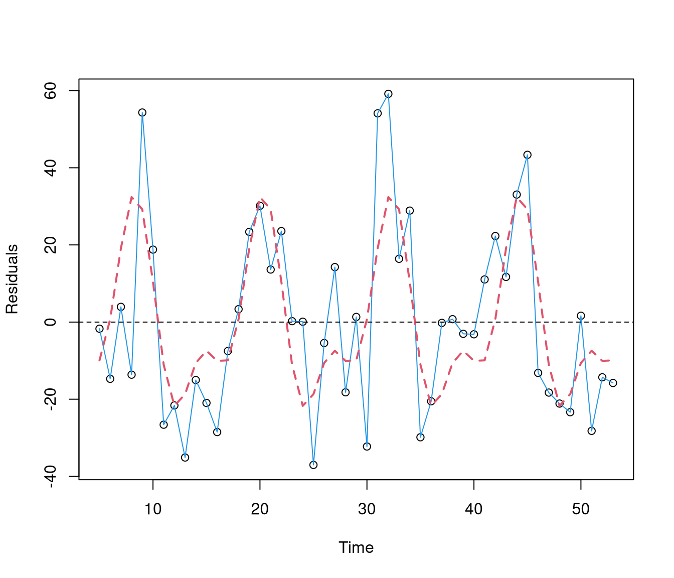
The extra sine and cosine pair gives a noticeably more flexible shape. It captures a steeper winter peak and a flatter period through part of the year without requiring a separate coefficient for each month.
33.3.4 Putting the Model Together
Electricity_lm6 <- lm(Bill ~ Days + Estimate + Guestwks + Time + SinTime + CosTime +
    Sin2Time + Cos2Time, data = Electricity)
summary(Electricity_lm6)
Call:
lm(formula = Bill ~ Days + Estimate + Guestwks + Time + SinTime +
    CosTime + Sin2Time + Cos2Time, data = Electricity)

Residuals:
    Min      1Q  Median      3Q     Max
-37.718  -9.495  -0.918   9.350  34.942

Coefficients:
            Estimate Std. Error t value Pr(>|t|)
(Intercept)  24.2994    35.3845   0.687   0.4962
Days          1.6721     1.2801   1.306   0.1989
Estimate     10.6697     7.0672   1.510   0.1390
Guestwks     11.0988     1.5241   7.282 7.62e-09 ***
Time          0.1432     0.1984   0.722   0.4745
SinTime      27.0035     4.0213   6.715 4.68e-08 ***
CosTime      -1.5594     3.6114  -0.432   0.6682
Sin2Time     -6.1630     3.4560  -1.783   0.0821 .
Cos2Time     -7.5589     3.6172  -2.090   0.0430 *
---
Signif. codes:  0 '***' 0.001 '**' 0.01 '*' 0.05 '.' 0.1 ' ' 1

Residual standard error: 16.84 on 40 degrees of freedom
Multiple R-squared:  0.7882,    Adjusted R-squared:  0.7458
F-statistic: 18.6 on 8 and 40 DF, p-value: 2.985e-11plot(Bill ~ Time, data = Electricity)
lines(Bill ~ Time, data = Electricity, col = 4)
lines(Electricity_lm6$fitted.values ~ Time, data = Electricity, col = 2, lwd = 2,
lty = 2)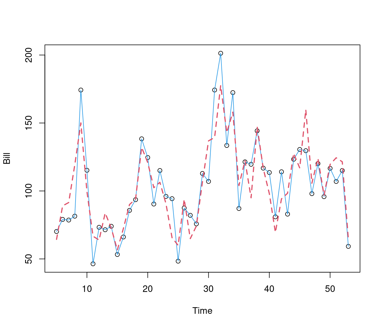
This final model is still a regression model. The main difference is that the seasonal predictors are now smooth waves rather than month indicators.
33.4 Fourier Terms in a Modern Example
The Seoul bike data use the same idea, but on a daily time scale. The sine and cosine terms are usually written more systematically as Fourier terms.
seoul_daily <- read_csv("../data/seoul_bike_daily.csv", show_col_types = FALSE) |>
    mutate(S1 = sin(2 * pi * day_index/365), C1 = cos(2 * pi * day_index/365), S2 = sin(4 *
        pi * day_index/365), C2 = cos(4 * pi * day_index/365))

seoul_daily |>
    head() |>
kable()| date | day_index | rented_bike_count | mean_temperature | mean_humidity | mean_wind_speed | mean_visibility | mean_dew_point_temperature | total_solar_radiation | total_rainfall | total_snowfall | season | holiday_any | functioning_day_all | S1 | C1 | S2 | C2 |
|---|---|---|---|---|---|---|---|---|---|---|---|---|---|---|---|---|---|
| 2017-12-01 | 1 | 9539 | -2.4541667 | 45.87500 | 1.5375000 | 1870.750 | -13.545833 | 5.97 | 0.0 | 0.0 | Winter | no | yes | 0.0172134 | 0.9998518 | 0.0344216 | 0.9994074 |
| 2017-12-02 | 2 | 8523 | 1.3250000 | 61.95833 | 1.7125000 | 1471.083 | -5.716667 | 6.33 | 0.0 | 0.0 | Winter | no | yes | 0.0344216 | 0.9994074 | 0.0688024 | 0.9976303 |
| 2017-12-03 | 3 | 7222 | 4.8750000 | 81.54167 | 1.6125000 | 455.750 | 1.883333 | 3.01 | 4.0 | 0.0 | Winter | no | yes | 0.0516197 | 0.9986668 | 0.1031017 | 0.9946708 |
| 2017-12-04 | 4 | 8729 | -0.3041667 | 52.50000 | 3.4500000 | 1362.833 | -9.925000 | 6.79 | 0.1 | 0.0 | Winter | no | yes | 0.0688024 | 0.9976303 | 0.1372788 | 0.9905325 |
| 2017-12-05 | 5 | 8307 | -4.4583333 | 36.41667 | 1.1083333 | 1959.458 | -17.425000 | 0.86 | 0.0 | 0.0 | Winter | no | yes | 0.0859648 | 0.9962982 | 0.1712931 | 0.9852201 |
| 2017-12-06 | 6 | 6669 | 0.0458333 | 70.79167 | 0.6958333 | 1186.875 | -5.187500 | 6.14 | 1.3 | 8.6 | Winter | no | yes | 0.1031017 | 0.9946708 | 0.2051045 | 0.9787401 |
seoul_fourier <- lm(rented_bike_count ~ day_index + S1 + C1 + S2 + C2 + mean_temperature +
    total_rainfall + total_solar_radiation, data = seoul_daily)
summary(seoul_fourier)
Call:
lm(formula = rented_bike_count ~ day_index + S1 + C1 + S2 + C2 +
    mean_temperature + total_rainfall + total_solar_radiation,
    data = seoul_daily)

Residuals:
     Min       1Q   Median       3Q      Max
-27475.5  -1526.5    474.7   2918.6  10393.4

Coefficients:
                       Estimate Std. Error t value Pr(>|t|)
(Intercept)            7852.642   1635.166   4.802 2.31e-06 ***
day_index                14.427      5.591   2.581  0.01026 *
S1                    -3429.607   1166.534  -2.940  0.00350 **
C1                    -3713.282   1069.412  -3.472  0.00058 ***
S2                    -1009.192    516.924  -1.952  0.05169 .
C2                     2766.476    421.357   6.566 1.84e-10 ***
mean_temperature        157.521     84.559   1.863  0.06330 .
total_rainfall         -201.256     29.827  -6.747 6.11e-11 ***
total_solar_radiation   373.863     60.035   6.227 1.34e-09 ***
---
Signif. codes:  0 '***' 0.001 '**' 0.01 '*' 0.05 '.' 0.1 ' ' 1

Residual standard error: 5410 on 356 degrees of freedom
Multiple R-squared:  0.728, Adjusted R-squared:  0.7219
F-statistic: 119.1 on 8 and 356 DF,  p-value: < 2.2e-16
seoul_daily |>
mutate(fitted = fitted(seoul_fourier)) |>
ggplot(aes(x = day_index, y = rented_bike_count)) + geom_line(alpha = 0.6) +
geom_line(aes(y = fitted), colour = "red", linewidth = 1) + labs(x = "Day index",
y = "Daily rented bike count", title = "Fourier terms give a smooth seasonal fit for bike demand")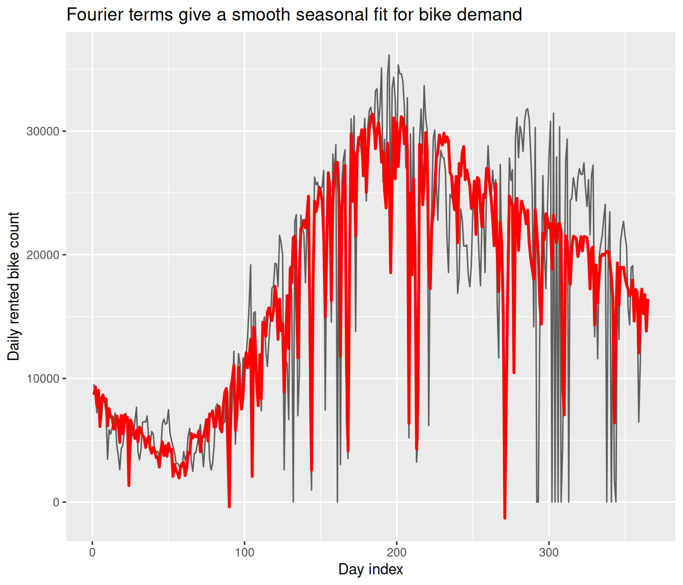
The electricity example introduced the ideas in a small, interpretable setting. The Seoul bike model shows the same method on a larger dataset, where the sine and cosine pairs become a compact way to represent annual seasonality.