31 Splines and LOESS: Flexible Regression Curves
31.1 Splines and LOESS: Flexible Regression Curves
So far we have focused on parametric regression models, where the mean response is described by a small number of coefficients. In this lecture we use the Seoul Bike Sharing data to study a different problem: the relationship between demand and weather is clearly nonlinear.
By the end of this lecture, students should be able to:
- Explain why a straight-line mean function can be too restrictive.
- Use LOESS to explore nonlinear structure.
- Fit regression splines using basis functions.
- Explain the difference between ordinary and natural splines.
- Recognise how added flexibility creates the need for regularisation.
31.1.1 Running Example: Hourly Bike Demand
Download seoul_bike_hourly.csv
# A tibble: 8,760 × 16
   date       datetime            day_index  hour rented_bike_count temperature
   <date>     <dttm>                  <dbl> <dbl>             <dbl>       <dbl>
 1 2017-12-01 2017-12-01 00:00:00         1     0               254        -5.2
 2 2017-12-01 2017-12-01 01:00:00         1     1               204        -5.5
 3 2017-12-01 2017-12-01 02:00:00         1     2               173        -6
 4 2017-12-01 2017-12-01 03:00:00         1     3               107        -6.2
 5 2017-12-01 2017-12-01 04:00:00         1     4                78        -6
 6 2017-12-01 2017-12-01 05:00:00         1     5               100        -6.4
 7 2017-12-01 2017-12-01 06:00:00         1     6               181        -6.6
 8 2017-12-01 2017-12-01 07:00:00         1     7               460        -7.4
 9 2017-12-01 2017-12-01 08:00:00         1     8               930        -7.6
10 2017-12-01 2017-12-01 09:00:00         1     9               490        -6.5
# ℹ 8,750 more rows
# ℹ 10 more variables: humidity <dbl>, wind_speed <dbl>, visibility <dbl>,
#   dew_point_temperature <dbl>, solar_radiation <dbl>, rainfall <dbl>,
#   snowfall <dbl>, season <chr>, holiday <chr>, functioning_day <chr>
The core question for this lecture is:
How does hourly bike demand change with temperature?
31.1.2 Why Go Beyond Straight Lines?
A straight-line model can underfit. A highly flexible curve can overfit. Our aim is to describe the mean relationship without losing the regression framing.
seoul_hourly |>
    ggplot(aes(x = temperature, y = rented_bike_count)) + geom_point(alpha = 0.06) +
    labs(x = "Temperature (C)", y = "Hourly rented bike count", title = "Bike demand changes nonlinearly with temperature")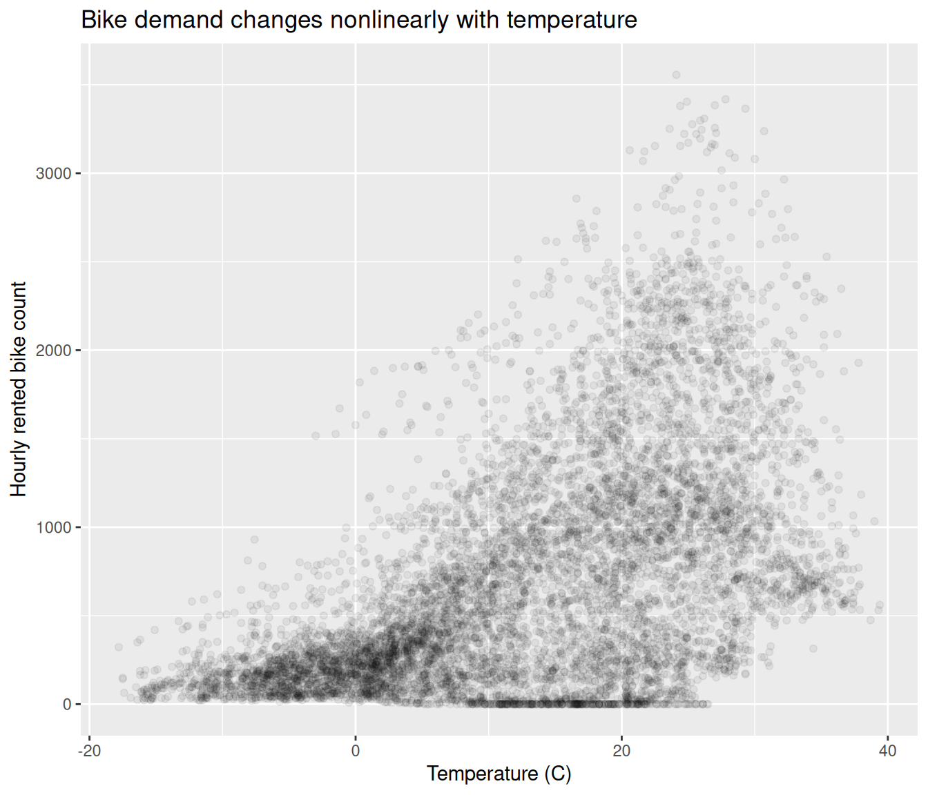
31.2 Example 1: LOESS
31.2.1 The LOESS Idea
LOESS fits many small local regressions instead of one global line.
- Choose a target point.
- Borrow nearby observations.
- Fit a weighted local regression.
31.2.2 LOESS with the Seoul Bike Data
seoul_hourly |>
    ggplot(aes(x = temperature, y = rented_bike_count)) + geom_point(alpha = 0.05) +
    geom_smooth(method = "loess", formula = y ~ x, span = 0.15, se = FALSE, linewidth = 1,
        aes(colour = "Span = 0.15", alpha = "Span = 0.15")) + geom_smooth(method = "loess",
    formula = y ~ x, span = 0.45, se = FALSE, linewidth = 1, aes(colour = "Span = 0.45",
        alpha = "Span = 0.45")) + scale_colour_manual(values = c(`Span = 0.15` = "green4",
    `Span = 0.45` = "blue")) + scale_alpha_manual(values = c(`Span = 0.15` = 0.8,
    `Span = 0.45` = 0.8)) + labs(x = "Temperature (C)", y = "Hourly rented bike count",
    colour = "LOESS span", alpha = "LOESS span", title = "LOESS span controls the smoothness of the fitted curve")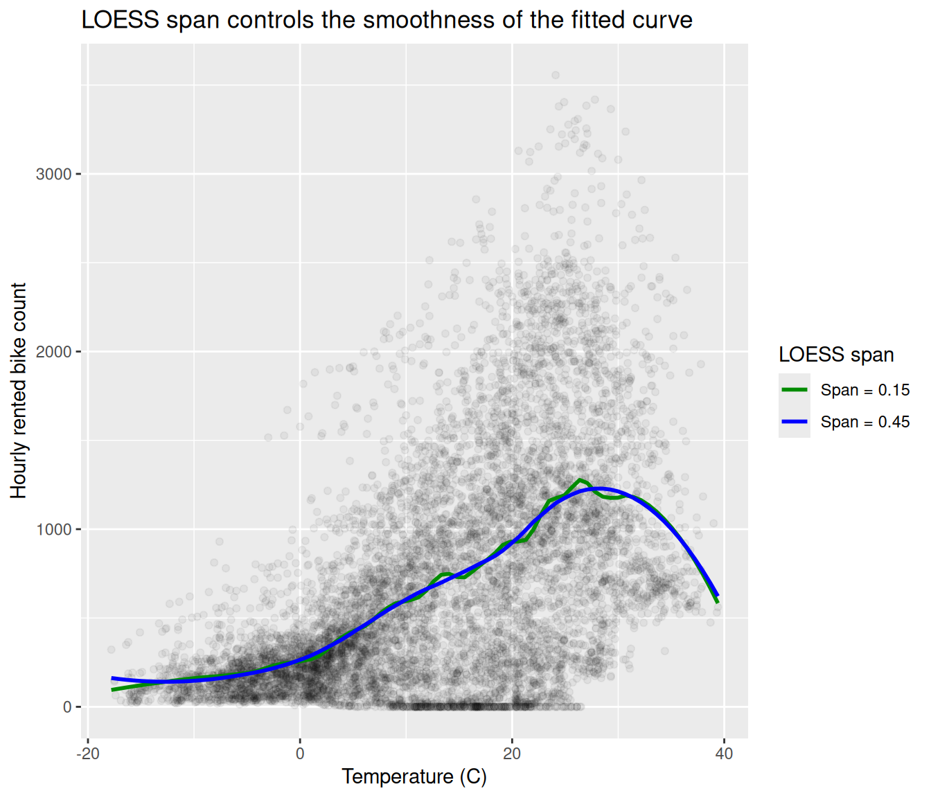
31.3 Example 2: Splines
31.3.1 The Key Conceptual Point
A spline model is still linear in its coefficients:
\[y = \beta_0 + \beta_1 b_1(x) + \beta_2 b_2(x) + \cdots + \beta_k b_k(x) + \varepsilon.\]
It is nonlinear in the original predictor, but linear in the unknown coefficients. That means we can still use standard regression tools.
31.3.2 Linear, Spline, and Natural Spline Fits
library(splines)

seoul_temp = seoul_hourly |>
    select(temperature, rented_bike_count) |>
    filter(is.finite(temperature), is.finite(rented_bike_count))

lm_linear = lm(rented_bike_count ~ temperature, data = seoul_temp)
lm_bs = lm(rented_bike_count ~ bs(temperature, df = 5), data = seoul_temp)
lm_ns = lm(rented_bike_count ~ ns(temperature, df = 5), data = seoul_temp)

temp_grid = tibble(temperature = seq(min(seoul_temp$temperature), max(seoul_temp$temperature),
    length.out = 250))

predictions = temp_grid |>
    mutate(Linear = predict(lm_linear, newdata = temp_grid), `B-spline` = predict(lm_bs,
        newdata = temp_grid), `Natural spline` = predict(lm_ns, newdata = temp_grid)) |>
    pivot_longer(cols = c(Linear, `B-spline`, `Natural spline`), names_to = "model",
        values_to = "fitted_bikes")

seoul_temp |>
    ggplot(aes(x = temperature, y = rented_bike_count)) + geom_point(alpha = 0.05) +
    geom_line(data = predictions, aes(x = temperature, y = fitted_bikes, colour = model,
        linetype = model, alpha = model), linewidth = 1) + scale_colour_manual(values = c(Linear = "red",
    `B-spline` = "blue", `Natural spline` = "forestgreen")) + scale_linetype_manual(values = c(Linear = "solid",
    `B-spline` = "dotted", `Natural spline` = "dotdash")) + scale_alpha_manual(values = c(Linear = 0.5,
    `B-spline` = 1, `Natural spline` = 1)) + labs(x = "Temperature (C)", y = "Hourly rented bike count",
    colour = "Model", linetype = "Model", alpha = "Model", title = "Splines allow flexible but still regression-based fits")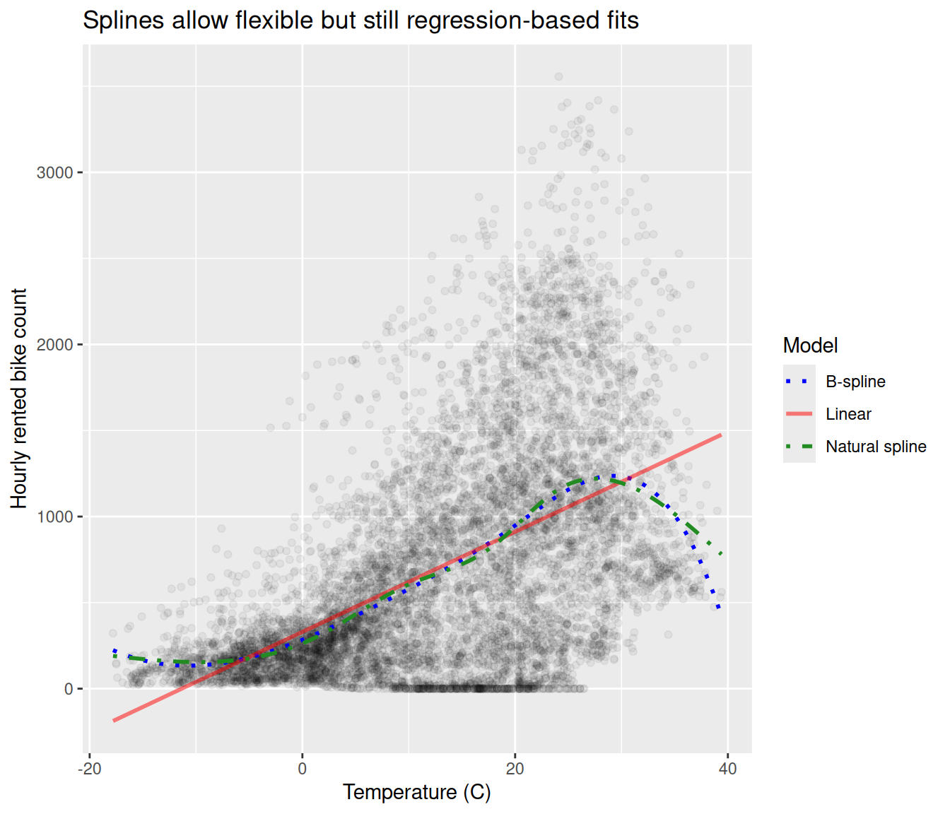
31.3.3 Natural Splines vs Ordinary Splines
predictions |>
    filter(model %in% c("B-spline", "Natural spline")) |>
    ggplot(aes(x = temperature, y = fitted_bikes, colour = model)) + geom_line(linewidth = 1) +
    labs(x = "Temperature (C)", y = "Fitted hourly bike count", colour = "Model",
        title = "Natural splines constrain the fit near the boundaries")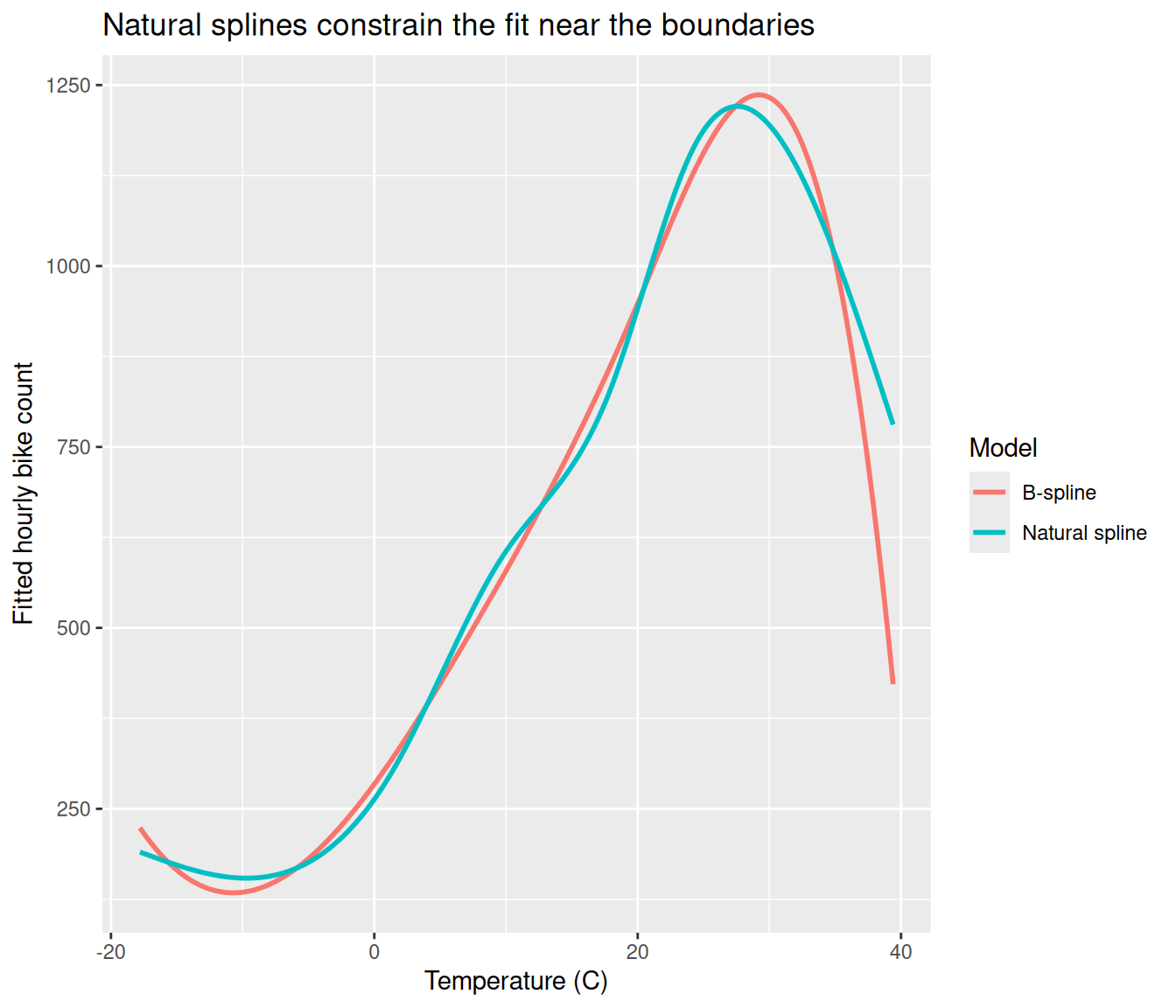
Natural splines are often a sensible default because we tend to trust the extremes of the predictor range less than the middle.
31.4 A Second Nonlinear Signal
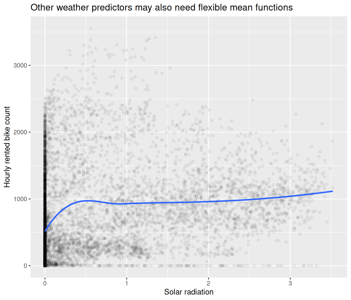
Temperature is not the only candidate for nonlinear modelling. Solar radiation may also have a curved relationship with demand.
seoul_hourly |>
    ggplot(aes(x = solar_radiation, y = rented_bike_count)) + geom_point(alpha = 0.05) +
    geom_smooth(method = "loess", formula = y ~ x, se = FALSE, linewidth = 1) + labs(x = "Solar radiation",
    y = "Hourly rented bike count", title = "Other weather predictors may also need flexible mean functions")